1 Introduction to Algorithms
1.1 Problems and Problem Instances
A problem \(P\) is a general class of questions to answer.
Problems are (infinite) families of general questions.
We call a version of the problem with specific values a problem instance \(I\) (or just instance).
Example 1.1 (Quadratic Equations) Finding the roots of a quadratic equation \(ax^2 + bx + c = 0\) is an example of a problem.
Finding the roots of a specific quadratic function is an instance of this problem. For example, finding \(x\) such that \(2x^2 + 8x + 5 = 0\) is a problem instance.
1.2 Algorithms
We are interested in finding procedures for solving every possible instance of a given problem. Such a procedure is called an algorithm.
Definition 1.1 (Algorithm) An algorithm for a given problem is a finite sequence of operations which return the correct solution for all problem instances.
Example 1.2 (An Algorithm for Quadratic Equations) We solve quadratic equations of the form \(ax^2 + bx + c = 0\) using the quadratic formula: \[ x = \frac{-b \pm \sqrt{b^2 - 4ac}}{2a}.\]
We can think of evaluating this formula as an algorithm consisting of the steps:
- Compute \(u:= b^2 - 4ac\).
- Compute \(v:= 2a\).
- Compute \(z := \sqrt{u} = \sqrt{b^2 - 4ac}\).
- Compute \[ x_1 = \frac{-b + z}{v}, \hspace{0.5in} x_2 = \frac{-b - z}{v}. \]
1.3 Goals of the Module
We are interested in:
Designing algorithms for solving specific problems.
Proving that a proposed algorithm produces correct solutions.
Complexity of algorithms: Analysing how long it takes for the algorithm to terminate, i.e., how many operations are required in general.
Complexity of problems: how long it may take to solve a problem, regardless of which algorithm is used.
1.4 Combinatorial Optimization
1.4.1 Combinatorial Optimization Problems
We will focus on combinatorial optimization problems: \[\min c(X) \text{ such that } X \in \mathcal{X},\] where \(c: \mathcal{X} \mapsto \mathbf{R}\) is a cost function and \(\mathcal{X}\) is a finite set of feasible solutions.
1.4.2 Solving Combinatorial Problems
Since \(\mathcal{X}\) is finite, we can always solve by complete enumeration: exhaustively calculating \(c(X)\) for each \(X \in \mathcal{X}\) to find one with minimum cost.
In practice, \(\mathcal{X}\) is extremely large and complete enumeration is prohibitively expensive.
In many cases, \(\mathcal{X}\) is defined implicitly as description and enumerating all possible solutions is a difficult task on its own.
We want faster, specialized algorithms exploiting mathematical structure of the given problem.
1.4.3 Examples of Combinatorial Problems
Combinatorial optimization is ubiquitous in operations research and management science1
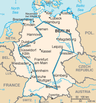
Example 1.3 (Travelling Salesperson Problem) Find a tour of shortest length visiting each location exactly once. Figure 1.1 gives an instance of the TSP and a solution where a tour of 15 cities in Germany is sought.
Example 1.4 (The Shortest Path Problem) Find shortest/minimum length route in network from origin to destination.
Example 1.5 (Knapsack/Assignment Problems) Find maximum value/minimum cost distribution of limited resources.
1.4.4 Types of Problems
We will focus on three primary forms of combinatorial optimization problems.
Definition 1.2 (Decision Problems) Given set \(\mathcal{X}\), cost \(c:\mathcal{X}\mapsto\mathbf{R}\) and scalar \(L \in \mathbf{R}\): \[\text{Determine if there is a } X \in \mathcal{X} \text{ with } c(X) \le L.\]
A decision problem takes problem instance defined by \(\mathcal{X}\), \(c\), and \(L\) as input. An algorithm for this problem would output Yes or No depending on the instance.
Definition 1.3 (Decision problem – Search version) Given \(\mathcal{X}\), \(c\), and \(L\) as input. Find \(X \in \mathcal{X}\) with \(c(X) \le L\).
Definition 1.4 (Optimization problem – Search version) Given \(\mathcal{X}\) and \(c\) as input. Find \(X \in \mathcal{X}\) minimizing \(c(X)\).
1.4.5 Exact and Approximation Algorithms
There are two primary classes of algorithms that we will consider: exact and approximation algorithms.
Definition 1.5 (Exact Algorithms) Exact algorithms provide an exact solution to the problem.
Definition 1.6 (Approximation Algorithms) Approximation Algorithms provide an approximate solution to the problem, but not the exact solution in general.
- An \(\alpha\)-approximate algorithm returns \(\tilde X\) within \(\alpha\)-ratio of optimal value: \(c(X^*) \le c(\tilde X) \le \alpha \cdot c(X^*),\) for some \(\alpha > 1\).
Aside from these two classes, we also have heuristics which provide potential solutions without guarantees of quality.
Definition 1.7 (Heuristics) Heuristic algorithms or heuristics provide solutions without guarantee of closeness to the optimal solution \(c(X^*)\).
1.4.6 Deterministic vs Random Algorithms
We can also classify algorithms based on whether steps are performed deterministically or at random.
Definition 1.8 (Deterministic Algorithms) Deterministic Algorithms follow the same series of steps for given input: \[ \text{{if A = B do X; else do Y}} \]
Definition 1.9 (Randomized Algorithms) Randomized algorithms have steps depending on random operations: \[\text{{Toss coin: if heads, do X; else do Y}}\]
A randomized exact/\(\alpha\)-algorithm may only return exact or \(\alpha\) solution within a certain probability.
1.4.7 Offline vs Online vs Robust Algorithms
Finally, we can further classify algorithms based on how they process information into problem instances.
Definition 1.10 (Offline Algorithm) The problem instance \(I\) is completely known at the beginning of the algorithm.
Definition 1.11 (Online Algorithm) The problem instance \(I\) is not completely known at start of the algorithm. Instead, the algorithm adapts to \(I\) as \(I\) unfolds over time.
Definition 1.12 Robust Algorithm: Instance \(I\) is not completely known at the beginning of the algorithm and it is not revealed over time.
The algorithm finds a solution that works for all possible realizations that \(I\) can take.
1.4.8 Example – Canadian Traveller Problem (CTP)
Shortest Path Problem with added complexity of not knowing which roads/routes are unavailable due to the weather beforehand2.
1.4.8.1 Deterministic/Off-line Version
We want to find the shortest or minimum length path in a network from origin to destination.
If the network routes are deterministic and are known then we have a deterministic exact algorithm for the shortest path problem. We’ll discuss this algorithm at length later in the term.
1.4.8.2 The Random Case
Let’s suppose that the routes are random or partially observed. For example, this could occur when inclement weather causes certain roadways to close, but they are not known until the road closure is encountered en route.
An online algorithm would find a partial path using known routes (so far), and then dynamically update the solution as conditions change or become known.
A robust algorithm would find a path/itinerary that works under any weather conditions.