10 Algorithms for (Potentially) Intractable Problems

Most real-world problems are either \(\mathbf{NP}\)-complete or \(\mathbf{NP}\)-hard (if not worse).

Unless \(\mathbf{P}=\mathbf{NP}\), we cannot solve these problems efficiently.

We still need an algorithm to solve them. Have two approaches:

Exponential-time enumeration algorithms.
Polynomial-time approximation algorithms.

10.1 Partial Enumeration

We can often (but not always) carefully apply enumeration to eliminate large numbers of potential solutions. We’ll illustrate using an instance of the satisfiability problem (SAT).

Example 10.1 Consider the following instance of SAT: \[\begin{align*} (Y_1 \vee Y_2 \vee Y_3 \vee Y_4) \wedge (Y_1 \vee -Y_2) \wedge (Y_2 \vee - Y_3) \\ \wedge (Y_3 \vee -Y_4) \wedge (Y_4 \vee - Y_1) \wedge (-Y_1 \vee - Y_4) \end{align*}\]

We can solve the problem by enumeration:

Build all possible combinations of T/F for the variables.
Check if any satisfy all of the clauses.

For Example 10.1, we have four variables, \(Y_1, Y_2, Y_3, Y_4\) to assign value \(T\) or \(F\) to. Since each variable takes one of two possible values, we have \[ 2^4 = 16 \] possible truth assignments.

In general, \(n\) variables, \(Y_1, Y_2, \dots, Y_n\), have \(2^n\) possible truth assignments. This clearly runs in exponential time. We cannot construct all possibilities and check if clauses are satisfied in a reasonable amount of time unless \(n\) is small.

10.1.1 Plans for Improvement

Let’s try to design an algorithm which does not consider every possible truth assignment.

This will still be exponential-time in worst case, but often faster the complete enumeration.

10.1.2 Partial Enumeration for SAT

Let’s consider the SAT instance given in Example 10.1: \[\begin{align*} (Y_1 \vee Y_2 \vee Y_3 \vee Y_4) \wedge (Y_1 \vee -Y_2) \wedge (Y_2 \vee - Y_3) \\ \wedge (Y_3 \vee -Y_4) \wedge (Y_4 \vee - Y_1) \wedge (-Y_1 \vee - Y_4). \end{align*}\] Let’s call this instance \((P_1)\).

Let’s consider the first variable \(Y_1\).

\(Y_1\) can take two values \(T\) and \(F\).
Can build two subinstances of SAT, one where \(Y_1 = F\) and \(Y_1 = T\).

10.1.2.1 Investigating \(Y_1 = F\)

If we set \(Y_1 = F\), then \((P_1)\) becomes \[ (F \vee Y_2 \vee Y_3 \vee Y_4) \wedge (F \vee -Y_2) \wedge (Y_2 \vee - Y_3) \wedge (Y_3 \vee -Y_4) \wedge (Y_4 \vee T) \wedge (T \vee -Y_4) \] after substituting \(Y_1 = F\) in each clause. We can simplify by:

dropping any \(F\) literals in clauses;
eliminating clauses with \(T\) literals, since these are already satisfied.

This yields the SAT instance \((P_2)\): \[ (Y_2 \vee Y_3 \vee Y_4) \wedge (-Y_2) \wedge (Y_2 \vee - Y_3) \wedge (Y_3 \vee -Y_4). \] It should be clear from inspection that there are no valid truth assignments with \(Y_2 = T\) and \(Y_1 = F\). Indeed, this would violate the clause \((-Y_2)\) in \((P_2)\). We’ll revisit this after investigating the case when \(Y_1 = T\).

10.1.2.2 Investigating \(Y_1 = T\)

Substituting \(Y_1 = T\) in \((P_1)\) and simplifying the clauses gives the new instance \((P_3)\) of SAT: \[ (Y_2 \vee - Y_3) \wedge (Y_3 \vee -Y_4) \wedge (Y_4) \wedge (-Y_4). \] Note that we cannot have \(Y_4 = T\) and \(Y_4 = F\). Thus, we must have \[ (Y_4) \wedge (-Y_4) = F \] and \((P_3)\) is infeasible. This implies that there are no solutions to \((P_1)\) with \(Y_1 = T\)! This eliminates half of the possible truth assignments that we need to consider.

10.1.2.3 Completing the Partial Enumeration

We can split \((P_2)\) into two subproblems by setting \(Y_2 = F\): or \(Y_2 = T\). We already saw that the problem \((P_5)\) we obtain by setting \(Y_2 = T\) is infeasible. On the other hand, after setting \(Y_1 = F\) and \(Y_2 = F\), we obtain the subproblem \((P_4)\): \[ (Y_3 \vee Y_4) \wedge (-Y_3) \wedge (Y_3 \vee - Y_4). \]

It is not obvious whether \((P_4)\) is feasible or infeasible, so we split again:

Setting \(Y_1 = F = Y_2\) and \(Y_3=F\) gives the subproblem \((P_6)\): \[ Y_4 \wedge (-Y_4), \] which is infeasible.
Setting \(Y_1 = F = Y_2\) and \(Y_3=T\) gives an infeasible subproblem because the clause \(-Y_3\) is not satisfied.

All subproblems are infeasible in the last step of our branching process. This implies that the original problem \((P_1)\) is infeasible. That is, we cannot satisfy all clauses with any assignment of \(T\) or \(F\) to the variables. Thus, we answer NO for this instance of SAT.

Note: we only needed to check \(6\) subproblems or possible truth assignments, which is much smaller than the \(16\) that full enumeration would consider.

10.1.3 Another Example

Example 10.2 Consider the following instance \((P_1)\) of SAT: \[ (-Y_1 \vee Y_2 \vee -Y_3) \wedge (Y_4 \vee -Y_2 \vee Y_3) \wedge (-Y_4 \vee Y_2 \vee Y_3). \] This is a YES-instance of SAT. Indeed, \((F, T, T, T)\) is a valid truth assignment (among others). We’ll use partial enumeration to solve this instance of SAT.

10.1.3.1 Branching using \(Y_1\)

Let’s branch on \(Y_1\) again, we obtain two subproblems \((P_2)\) and \((P_3)\) by assigning the value \(Y_1 = F\) and \(Y_1 = T\), respectively: \[\begin{align*} (Y_4 \vee -Y_2 \vee Y_3) \wedge (-Y_4 \vee Y_2 \vee Y_3) && && (P_2) \\ (Y_2 \vee -Y_3) \wedge (Y_4 \vee -Y_2 \vee Y_3) \wedge (-Y_4 \vee Y_2 \vee Y_3). && && (P_3) \end{align*}\] It is not immediately clear if \((P_2)\) or \((P_3)\) are YES-instances of SAT, so we need to branch further.

10.1.3.2 Solving \((P_2)\)

Let’s focus on \((P_2)\) to start. We assume that \(Y_1 = F\) and set \(Y_2 = T\) or \(Y_2 = F\):

If \(Y_2 = T\) then we obtain the subproblem \((P_4)\): \[ (Y_4 \vee Y_3). \] This is clearly a YES-instance of SAT: setting \(Y_4 = T\) and/or \(Y_3 = T\) satisfies the clause.
If \(Y_2 = F\), then we obtain the subproblem \((P_5)\) \[ (-Y_4) \vee Y_3 \] which is also a YES-instance of SAT. Indeed, \(Y_4 = F\) and/or \(Y_3 = T\) satisfies the clause.

This implies that \((P_1)\) is also a YES-instance of SAT: \[ (F,T, T, T), (F,T,T,F), (F,T,F,T), (F,F,F,F), (F,F,F,T) \] are all solutions of \((P_1)\).

At this point, we can conclude that \((P_1)\) is a YES-instance of SAT and stop the algorithm.

10.1.3.3 Solving \((P_3)\)

For illustrative purposes, let’s apply branching to \((P_3)\) as well:

Assuming \(Y_2 = T\) gives \[ (Y_3 \vee Y_4); \] this implies that \((T, T, T, T/F)\) and \((T, T, T/F, T)\) are solutions of \((P_1)\).
On the other hand, if \(Y_2 = F\), we have \[ - Y_3 \wedge (-Y_4 \vee Y_3 ). \] This implies that \((T, F, F, F)\) is a solution of \((P_1)\).

10.2 Branch and Bound for CLIQUE

Recall the CLIQUE problem:

CLIQUE: Given an undirected graph \(G=(V,E)\), find a clique of maximum size.

10.2.1 Characteristic Vectors

Definition 10.1 Let \(C\) be a clique (or, more generally, subset of \(V\)) for graph \(G = (V,E)\). The characteristic vector of \(C\) is the binary vector such that \[ x_i = \begin{cases} 1, & \text{if } i \in C, \\ 0, & \text{if } i \notin C. \end{cases} \]

Figure 10.1: Graph \(G\) with clique \(C = \{0,2,3\}\)

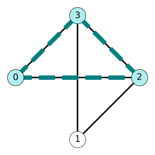
Example 10.3 Consider the graph \(G\) with clique \(C = \{0,2,3\}\) given in Figure 10.1. The characteristic vector \(x\) of \(C\) is \[ (x_0, x_1, x_2, x_3) = (1,0,1,1). \]

10.2.2 Partial Enumeration for CLIQUE

We can solve CLIQUE using complete enumeration, trying all possible 0/1 values for potential characteristic vectors \(x\).

We would need to consider \(2^n\) possible solutions for a instance with \(n\) vertices.

As with SAT we can create subinstances by setting \(x_j =1\) and \(x_j = 0\).

We are solving an optimization problem, so we need to exclude subinstances that yield suboptimal solutions. (This differs from SAT where we eliminated infeasible branches)

10.2.3 Branch and Bound Algorithms

Our partial enumeration algorithm for CLIQUE will take the form of a branch and bound algorithm.

Let’s introduce three values associated with each sub-instance \(I\):

lower bound \(LB(I)\): value of a feasible solution to subinstance \(I\).
upper bound \(UB(I)\): value larger than any optimal solution to \(I\).
global lower bound \(GLB\): value of the best feasible solution found so far.

We’ll use these to prune or ignore certain subinstances to allow partial enumeration.

10.2.3.1 Estimating Upper Bound for CLIQUE

A simple upper bound for clique is given by \[ UB(I) := |\{j\in V\}: x_j(I) = 1| + |\{j \in V\}: x_j(I) = -|. \] (Here ``\(-\)” denotes that the corresponding node can take value \(1\) or \(0\) in a possible solution.)

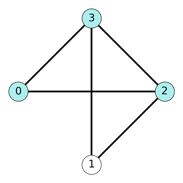
Example 10.4 Consider the graph \(G\) given in Figure 10.2.

In Figure 10.2 (a), node \(1\) is unassigned to the subset (it could be included or not), and the remaining nodes are included in the given set. Using the formula gives \[ UB(I) =|\{j\in V\}: x_j(I) = 1| + |\{j \in V\}: x_j(I) = -| = 3 + 1 = 4. \] On the other, the given set forms a clique, so we have \[ LB(I) = 3. \] This implies that the maximum clique for this graph contains either \(3\) nodes or \(4\) nodes.
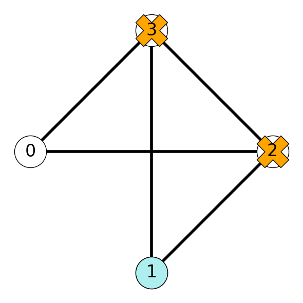
On the other hand, the sub-instance given in Figure 10.2 (b), assumes that nodes \(2\) and \(3\) are not included in a maximum clique, and node \(1\) is. In this case, we have \[ UB(I) = 1 + 1 = 2, \hspace{0.25in} LB(I) = 1. \] Note that this upper bound is less than the lower bound given by the sub-instance in Figure 10.2 (a). This implies that we do not need to further explore the sub-instance given in Figure 10.2 (b).

10.2.3.2 Pruning

Efficient branch and bound algorithms rely on pruning some nodes.

If \(UB(I) \le GLB\) then sub- instance \(I\) can be discarded or pruned.

The best \(I\) can give us is a solution with value \(UB(I)\), which is no better than the best solution found so far.

Example 10.5 Suppose that we have a solution of value \(3\) so that \(GLB =3\).

Let’s reconsider the sub-instance \(I\) given in Figure 10.2 (b). We can prune this branch because we know that it will not contain the maximum clique.

10.2.4 An Example of Solving CLIQUE using B+B

Consider the instance of clique given by

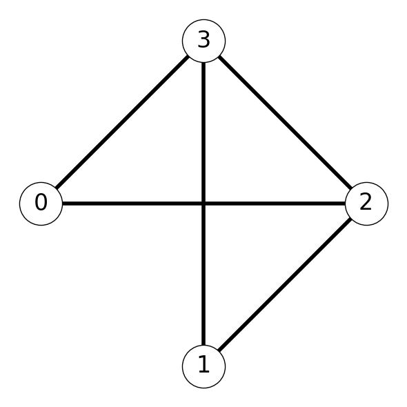
Let’s call this initial instance \(I_0\).

We initialize the branch and bound process with initial solution \(x = (-,-,-,-)\). This notation indicates that we assume that any of the four nodes can be included in a maximum clique; we’ll determine which ones will be. Our initial upper bound is \(4\) and the initial lower bound is \(0\).

We can obtain two sub-instances of CLIQUE by setting \(x_0 = 0\) or \(1\). We call these sub-instances \(I_1\) and \(I_2\) respectively.

10.2.4.1 Solving \(I_1\)

Let’s assume that \(x_0=1\). That is, that node \(0\) is included in a maximum clique:

We can update the lower bound \(LB = 1\) since \(\{0\}\) is a clique;
\(UB = 4\) is unchanged.

10.2.4.2 Branching on \(x_1\)

We can branch further by assuming that node \(1\) does or does not belong to a maximum clique, i.e., that \(x_1 = 1\) or \(x_1 = 0\).

If \(x_1 = 1\), then we are assuming that both nodes \(0\) and \(1\) belong to a clique. However, \(0\) and \(1\) are not adjacent. Therefore, this branch, \(I_3\), is infeasible. We cannot any set containing both nodes \(0\) and \(1\) cannot be a clique.
If \(x_1 = 0\), then we assume that Node \(0\) belongs to a maximum clique, but Node \(1\) does not. This yields sub-instance \(I_4\) We have \[ LB = 1, \hspace{0.25in} UB = 3 \] in this case.

10.2.4.3 Solving \(I_4\)

We can split \(I_4\) further, but setting \(x_2 = 1\) or \(x_2 = 0\):

If \(x = (1, 0, 1, -)\), then we have found at least a clique \(\{0,2\}\) of size \(2\) since \(\{0,2\} \in E\). This implies gives bounds \[ LB = 2, \hspace{0.25in} UB = 3. \] Notice that our greatest lower bound so far is \(GLB = 2\). Let’s call this sub-instance \(I_5\).
If \(x =(1,0,0,-)\) then we have \(UB = 2 \le GLB\). Therefore, this set contains, at best, a clique of size \(2\). Therefore, we can prune this subinstance \((I_6)\).

10.2.4.4 Solving \(I_5\)

\(I_7\): If we set \(x_3 = 1\), we obtain the solution \(x = (1,0,1,1)\). This corresponds to the clique \(\{0,2,3\}\). This is the largest clique we have found so far: \(GLB = 3\).

\(I_8\): On the other hand, taking \(x_3 = 0\) gives the clique \(\{0,2\}\) with two nodes (not a maximum clique).

10.2.4.5 Returing to \(I_2\)

We have successfully identified the largest clique containing node \(0\). We still need to investigate all vertex sets not containing node \(0\).

Let’s branch using \(x_1\):

Setting \(x_1 = 1\) gives sub-instance \(I_9\) with \(x = (0,1,-,-)\) Here, \(UB = 3 \le GLB\). We can prune this branch.
Setting \(x_1 = 0\) gives \(I_{10}\) with \(x = (0,0,-,-)\). Again, \(UB < GLB\) and we prune this branch.

10.2.4.6 Termination

We have now exhausted all possible solutions and have found maximum clique \(\{0,2,3\}\).

Note that if we had explored sub-instance \(I_2\) first (instead of \(I_1\)), we would have found the maximum clique \(\{1,2,3\}\) in the pruned branch \(I_9\).

10.3 Approximation Algorithms

We conclude by investigating algorithms for approximating the solution of intractable optimization problems.

We’ll focus on a variant of the travelling salesperson problem as an illustrative example.

10.3.1 Metric Undirected TSP

Definition 10.2 (Metric Undirected Travelling Salesperson Problem (MUTSP)) Given a complete undirected graph \(G=(V,E)\) with edge cost function \(c\) satisfying the triangle inequality:

\[ c_{ij} \le c_{ik} + c_{kj} \text{ for all } i,j,k \in V. \]

MUTSP: Find a Hamiltonian cycle of minimum total cost.

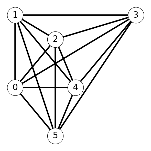
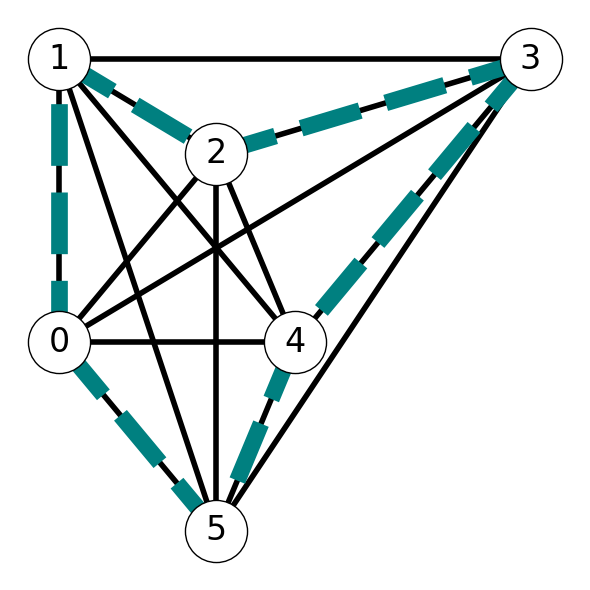
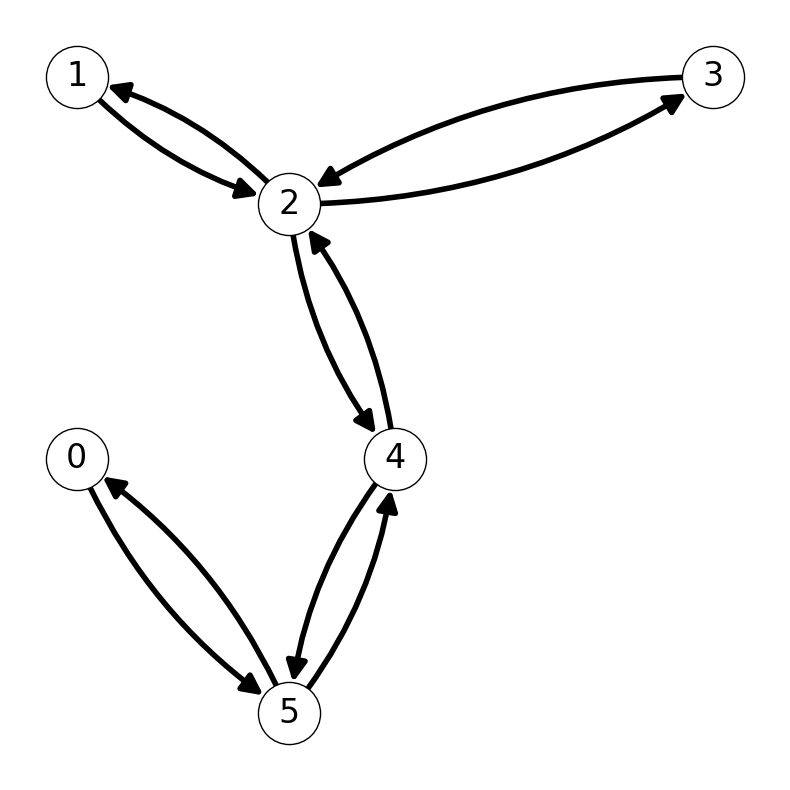
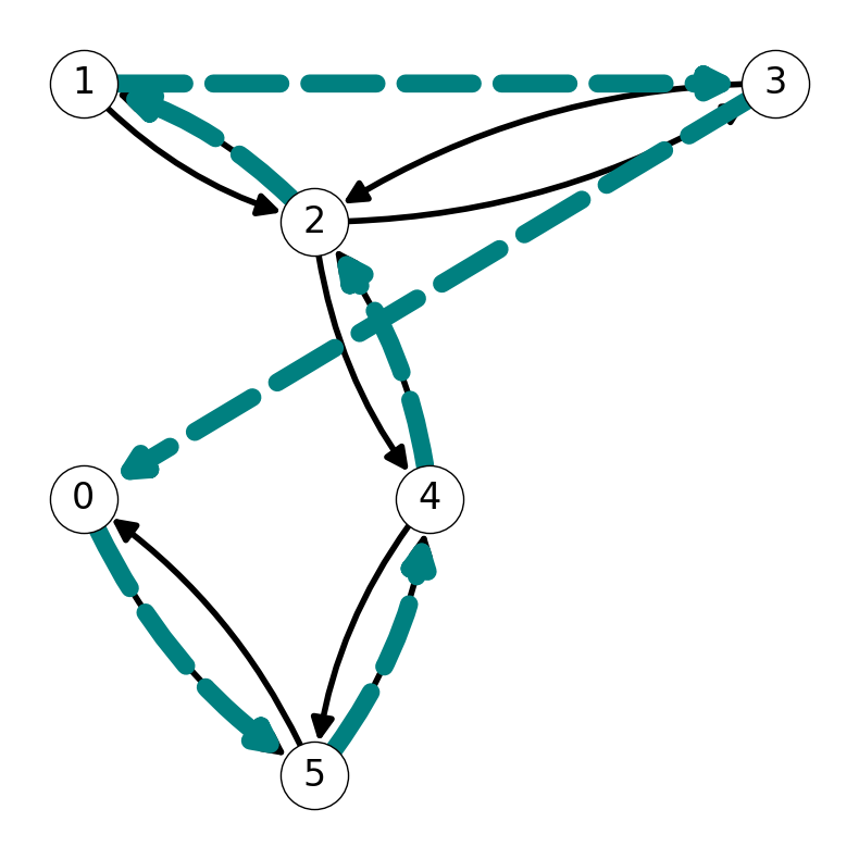
Example 10.6 Consider the graph \(G\) given in Figure 10.4 (a). Assume that \(c_{ij}\) is equal to the length of line segment representing edge \((i,j)\). The minimum cost Hamiltonian cycle is indicated by the highlighted edges in Figure 10.4 (b)

10.3.2 An Approximation Algorithm for MUTSP

10.3.2.1 Plan

We could develop a branch and bound algorithm for MUTSP similar to that we saw earlier for CLIQUE.

Instead, we develop an approximation algorithm. That is, we want an algorithm that:

Runs in polynomial time.
Always produces a feasible solution which is no more than \(\alpha\) times large than optimal value for some constant \(\alpha\).

10.3.2.2 Relaxing MUTSP

An optimal Hamiltonian cycle is a subset of edges that:

consists of a single cycle;
visits each vertex in \(V\) once;
has minimum cost.

Let’s relax the problem by ignoring the 1st constraint for now:

Find a subgraph satisfying (2) and (3). This may not be a cycle.
This is an instance of the minimum-cost spanning tree (MST) problem.

The feasible region of MST is larger than MUTSP. That is, every Hamiltonian cycle corresponds to a spanning tree. Indeed, deleting a single edge from a Hamiltonian cycle gives a spanning tree. However, not every spanning tree corresponds to a Hamiltonian cycle. Therefore: \[ \text{optimal MUTSP cost } \ge \text{optimal MST cost}. \]

This leads to two natural questions:

Can we use the MST to a obtain a feasible solution for MUTSP?
How are the values of these solutions related?

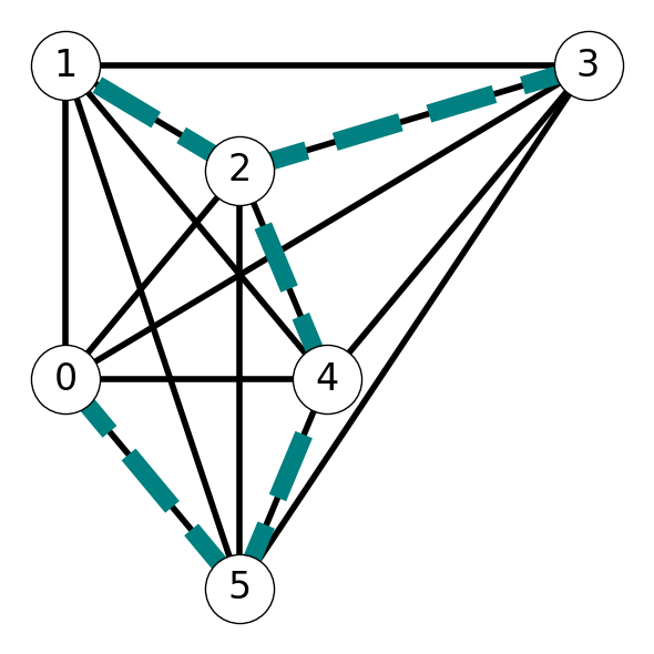
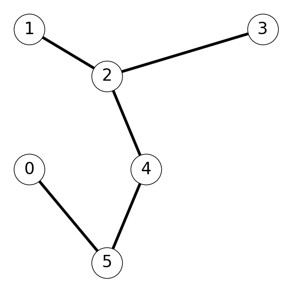
Example 10.7 Let’s revisit the graph \(G\) given in Figure 10.4 (a) (also given in Figure 10.5 (a)). This graph has minimum spanning tree \(T\) indicated in Figure 10.5 (b).

10.3.2.3 Building a Tour from a Tree

We can always construct a tour from the minimum spanning tree. - Indeed, choose a cycle that visits all vertices in \(G\) by traversing MST in some order.

This gives a tour using each MST each exactly twice. However, this tour is not simple.
We use each edge in the MST twice, so the total cost of this cycle is \[ 2 \times \text{ optimal MST cost}. \]

Example 10.8 Figure 10.4 (a) illustrates this process for the graph \(G\) considered in Example 10.6. The minimum spanning tree is given in Figure 1 (a). The cycle \[ C = (0,5,4,2,1,2,3,2,4,5,0) \] traverses every node and arc in \(G\) exactly twice (see Figure 10.7 (a)).

10.3.2.4 Finding a Simple Tour

We can produce a simple tour, i.e., a Hamiltonian cycle from the tour given by the minimum spanning tree:

Follow the edges of the not-simple tour until we reach a vertex for the second time.
Jump to the next unvisited node. Jump to the initial node if there are no unvisited nodes.

Note that this is always possible because \(G\) is complete.

Example 10.9 Let’s consider the graph \(G\) again. We saw in Example 10.8 that \[ C = (0,5,4,2,1,2,3,2,4,5,0) \] is a non-simple tour of \(G\). Traversing this cycle until we reach \(1\), then skipping to the unvisited node \(3\) along edge \(\{1,3\}\), then jumping back to \(0\) via edge \(\{3,0\}\) gives the Hamiltonian cycle \[ H = (0,5,4,2,1, 3, 0). \]

(a) The not-simple tour \(C\) given by \(T\)

10.3.2.5 Cost of this Hamiltonian Cycle

Recall that the cost function is metric:

skipping an intermediate node \(k\) on path from \(i\) to \(j\) does not increase the cost of the tour: \[ c_{ij} \le c_{ik} + c_{kj}. \] This implies that the cost of the Hamiltonian cycle computed using the MST has cost at most \(2\) times the cost of the minimum spanning tree.

Example 10.10 In our example, the cost of the Hamiltonian cycle is \[ c(H) = c_{05} + c_{54} + c_{42} + c_{21} + c_{13} + c_{30}. \] However, this graph is metric, so \[\begin{align*} c_{13} & \le c_{12} + c_{23} \\ c_{30} & \le c_{32} + c_{24} + c_{45} + c_{50}. \end{align*}\] This implies that we have \[ c(H) \le c(C) = 2 c(T). \]

10.3.2.6 Summary

In general, this process gives a Hamiltonian cycle \(H\) with cost \[ c(H) \le 2 c(T). \] However, we know that \[ c(T) \le \text{MUTSP optimal value}. \] This implies that \[ c(H) \le 2 \times \text{MUTSP optimal value}. \]

This shows that this algorithm always productes a feasible Hamiltonian cycle with value at most twice the optimal cost. Moreover, the algorithm runs in polynomial time since MST can be solved and we can construct the Hamiltonian cycle from the MST in polynomial time. Therefore, we have a 2-approximate algorithm for MUTSP (\(\alpha=2\)).

10.3.3 TSP in the Non-Metric Case

Theorem 10.1 TSP does not admit an approximation algorithm unless \(\mathbf{P}=\mathbf{NP}\).

Proof Idea: Use reduction to show that the existence of an \(\alpha\)-approximate algorithm for TSP would given an algorithm for any \(\mathbf{NP}\)-complete problem for all \(\alpha\ge 1\).