4 Complexity
4.1 Big-\(O\) Notation
Definition 4.1 (Big-\(O\) Notation) Given \(f,g:\mathbf{R}\mapsto\mathbf{R}\), we say \[f = O(g),\] i.e., \(f\) is of order \(g\), if there are \(n_0\) and \(c\in \mathbf{R}_+\) such that \[f(n) \le c~g(n) \hspace{0.15in} \text{for all } n \ge n_0.\]
Big-\(O\) notation captures the asymptotic behaviour of a function \(f\) when compared to another function \(g\).
4.1.1 Properties of Big-\(O\) Notation
Let \(f\) and \(g\) be positive functions \((f,g: \mathbf{R}\mapsto\mathbf{R}_+)\).
If \(\displaystyle \lim_{n\rightarrow \infty} \frac{f(n)}{g(n)}= \ell \in (0, \infty)\) then \[ f = O(g) \text{ and } g = O(f). \] For example, \(f(n) = 2n\) and \(g = 3n + \sqrt{n}\) satisfy \(f=O(g)\) and \(g=O(f)\).
If \(\displaystyle\lim_{n\rightarrow \infty} \frac{f(n)}{g(n)} = 0\) then \[ f = O(g) \text{ but } g \neq O(f). \] For example, \(f(n)=n\) and \(g(n) = 3n^3 + 2n\) satisfy \(f=O(g)\), but \(g \neq O(f)\).
Multiplicative and additive constants can be ignored: \[ a f(n) + b = O(f(n)). \] For example, \(f(n) = 5n^2 + 2 = O(n^2)\).
Lower order terms can be ignored: if \(g = O(f)\) then \[ f(n) + g(n) = O(f(n)). \] For example, \(6n^4 + e^n = O(e^n)\).
4.2 Elementary Operations and Computational Complexity
4.2.1 Computational Complexity
We can count the number of elementary operations or EOs carried out by an algorithm:
Arithmetic operations
Accesses to memory
Writing operations, etc.
Let \(f_A(n)\) and \(f_B(n)\) be the number of EOs required in worst case (the instance that requires the most EOs) by algorithms \(A\) and \(B\) to solve \(P\) with instance size \(n\).
Definition 4.2 We call \(O(f_A)\) and \(O(f_B)\) the computational complexity of \(A\) and \(B\). We choose \(O(f_A)\) and \(O(f_B)\) to be as small as possible.
4.2.2 The Cobham-Edmonds Thesis (1965)
We say that problem \(P\) is tractable or well-solved if:
There is an algorithm \(A\) for solving \(P\);
\(A\) has polynomial computational complexity.
4.2.3 Converting EOs and Run-Time
If each EO takes \(1\) \(\mu s\) (1 microsecond):
| \(n\) | \(f_A(n) = n^2\) | \(f_A(n) = 2^n\) |
|---|---|---|
| \(10\) | \(0.1~\text{ms}\) | \(1~\text{ms}\) |
| \(20\) | \(0.4~\text{ms}\) | \(1.0~\text{s}\) |
| \(30\) | \(0.9~\text{ms}\) | \(17.9\text{ min}\) |
| \(40\) | \(1.6~\text{ms}\) | \(12.7\text{ days}\) |
| \(50\) | \(2.5~\text{ms}\) | \(35.7\text{ years}\) |
| \(60\) | \(3.6~\text{ms}\) | \(366\text{ centuries}\) |
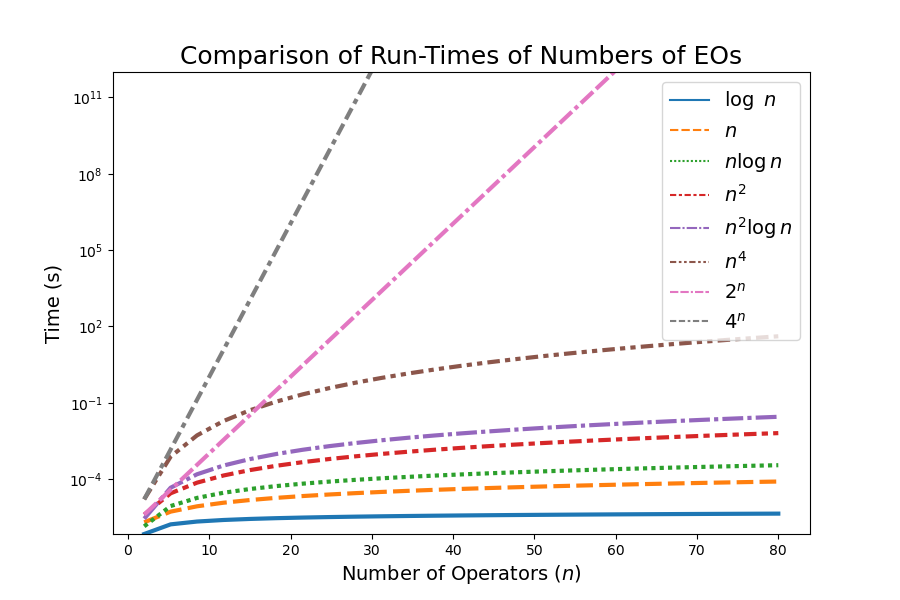
4.2.4 A Comparison of Complexity and Scaling
Assume again that each EO requires \(1~\mu\text{s}\).
The following figure compares how complexity scales as a function of \(n\) for
- logarithmic,
- polynomial,
- polylogarithmic, and
- exponential functions.
4.3 Examples
4.3.1 Complexity of Solving Quadratic Equations
Recall the following algorithm for solving quadratic equation \(ax^2 + bx + c = 0\):
Compute u = b*b - 4*a*c

Compute v = 2*a

Compute w = sqrt(u)

Compute x_plus = -(w - b)/v

Compute x_minus = - (w + b)/v
Let’s count the number of operations used in each step of the algorithm:
Computing
urequires 3 products and one subtraction (4 arithmetic operations total).Computing
vrequires 1 product.Computing
wrequires 1 call to thesqrtfunction, which uses a finite number of arithmetic operations. Let’s treat this as 1 operation for the purposes of estimating the complexity of applying the quadratic formula.Each of
x_plusandx_minusrequire 3 arithmetic operations.
The total number of arithmetic operations used by the quadratic formula is \(12 = O(1)\).
4.3.2 Complexity of Graph Reachability
Let’s analyse the complexity of the graph reachability algorithm given below:
Initialize Q = {s} and M = {}.

while Q != {}:

    # select a node i in Q
    Q = Q - {i} # remove i from Q.

    for j in L(i): # j is adjacent to i.

        if (j not in M) and (j not in Q):
            Q = Q + {j} # add j to Q.

    M = M + {i} # add i to M.
Let’s first count the number of operations need for each iteration of the algorithm:
Choosing a node
iinQ, removingifromQ, and addingitoMrequires \(O(1)\) operations each.The loop iterating over the adjacency list \(L(i)\) runs \(|L(i)| \le n-1\) times. Each occurence of the loop code uses \(O(1)\) operations.
We perform \(|Q| \le |V| = n\) steps of the outer-most loop.
Therefore, we have the upper bound on complexity \[ O(n(n-1)) = O(|E|). \]
4.3.2.1 An Improved Estimate
The steps of the inner for loop is executed for each node \(i\) at most once. This implies that each arc \((i,j)\) is explored at most once. Therefore, the steps of this loop are executed at most \(m\) times total.
This implies that the total complexity is \[ O(m) + O(n) = O(m+n). \] This is much smaller than the previous estimate if the graph is sparse, i.e., \(O(m) << O(n(n-1))\).