5 The Shortest Path Problem
5.1 Preliminaries
Definition 5.1 (The Shortest Path Problem – Unrestricted Lengths (SPP-U)) Given a directed graph \(G = (V,A)\) with:
two nodes \(s\) and \(t\);
length function \(\ell:A \mapsto \mathbf{R}\) (unrestricted in sign).
Find an \((s,t)\)-path with minimum total length.
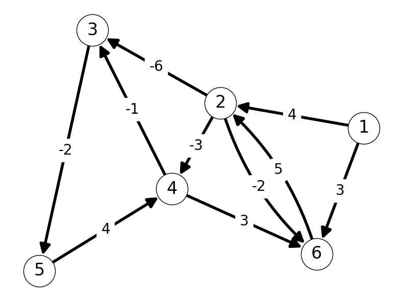
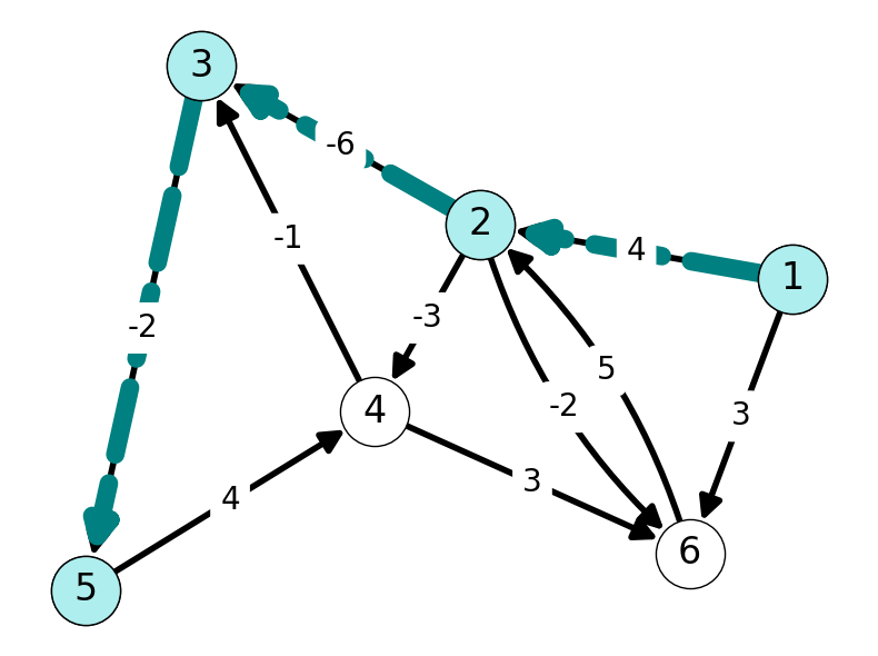
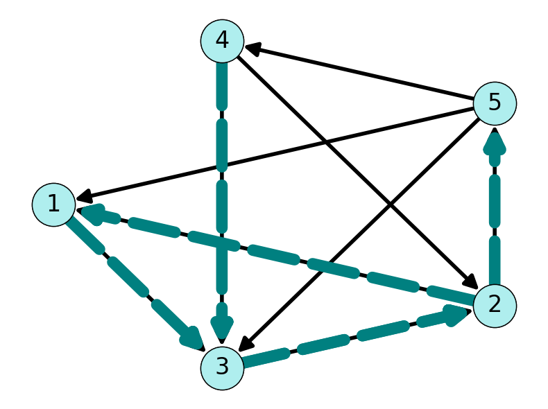
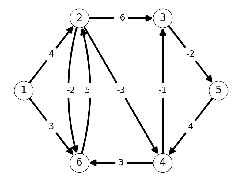
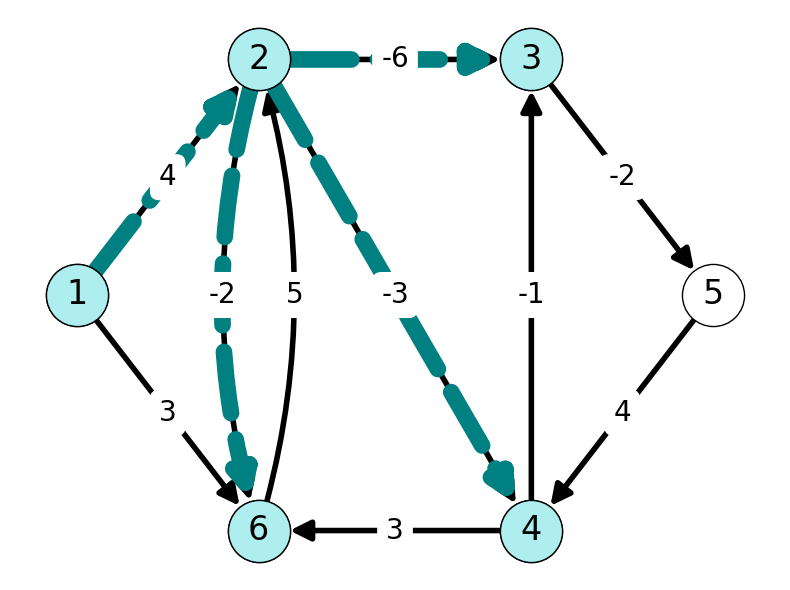
Example 5.1 Consider the graph given in Figure 5.1 (a). The shortest \((1,5)\)-path in this graph is \((1,2,3,5)\) with value equal to \[ \ell_{12} + \ell_{23} + \ell_{35} = 4 -6 -2 = -4. \]
5.1.1 Applications
5.1.1.1 Logistics and Transportation
In this field, we want to find \((s,t)\)-paths minimizing:
Travel time; \(\ell_{ij}\) is average time traveling along arc \((i,j)\).
Fuel consumption.
Likelihood of delays; etc.
5.1.1.2 Minimum Cardinality Path
We can find a path with minimum number of arcs by assigning \(\ell_{ij} = 1\) for all \((i,j)\in A\).
5.1.1.3 Component of Other Algorithm
SPP appears as a subproblem when solving other combinatorial optimization problems (more details later).
5.1.2 Simple Paths and Cycles
Definition 5.2 An \((s,t)\)-path \(P\) is simple if it does not visit the same node twice.
Note: if \(P\) visits the same node twice then \(P\) must contain at least one cycle.
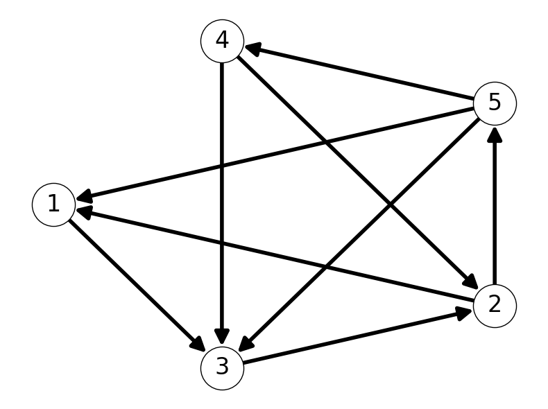
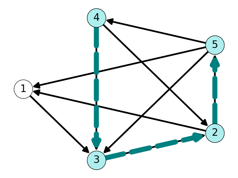
Example 5.2 Figure 5.2 gives an example of a simple path and a not simple path within a directed graph.
5.1.3 Unboundedness and Negative Cycles
Theorem 5.1 Suppose that \(G\) contains an \((s,t)\)-path \(P\) with a negative length cycle. Then SPP-U is unbounded.
Proof. Suppose that \(C\) is a negative length with length \[ \ell_{C} = \sum_{ij \in C} \ell_{ij} < 0. \]
Suppose further that \(P\) is an \((s,t)\)-path that traverses \(C\) exactly \(k\) times for some integer \(k> 0\). That is, \(C\) is contained in \(P\) exactly \(k\) times.
We can always augment this path to get a path with strictly smaller length. Indeed, consider the path \(\tilde P\) which contains all arcs of \(P\), but traverses \(C\) exactly \(k+1\) times. Then the length of \(\tilde P\) satisfies \[ \text{length }\tilde P = \text{length } P + \ell_C < \text{length } P \] since \(\ell_C < 0\).
Theorem 5.2 If no \((s,t)\)-path contains a negative-length cycle, then \(G\) admits a simple shortest \((s,t)\)-path.
If no \((s,t)\)-path in \(G\) contains a negative length cycle, then we can solve the SPP-U by restricting our search to simple paths.
Proof. Let \(P\) be a shortest \((s,t)\)-path in \(G\). Let’s also assume that every cycle \(C\) in \(P\) has nonnegative length \(\ell_C \ge 0\).
Let’s assume that \(P\) contains a cycle \(C\) starting and ending with node \(u\). That is, we can think of \(P\) as the union of the directed \((s,u)\)-path \(P_{su}\), the cycle \(C\), and the \((u,t)\)-path \(P_{ut}\). Let \(\ell^*\) denote the value of this path.
Now consider the \((s,t)\)-path given by following \(P_{su}\) to \(u\), then \(P_{ut}\) to \(t\). This is the path obtained by removing \(C\) from \(P\). This gives an \((s,t)\)-path with length \[ \ell^* - \ell_C \le \ell^*. \] Thus, removing cycle \(C\) from \(P\) does not increase the length of the path. We can repeat this process until we have obtained a simple path with minimum path length \(\ell^*\), or we obtain a simple path with length strictly less than \(\ell^*\) (a contradiction).
Example 5.3 To illustrate this phenomena, consider the graph given in Figure 5.3. This graph has \((1,5)\)-path \((1,2,3,4, 2,5)\) with length \(5\) (assuming all arcs have length \(1\)). However, this path contains the cycle \(C= (2,3,4,2)\). Removing the cycle \(C\) gives the shorter \((1,5)\)-path \((1,2,5)\) (with length \(2\)).
5.2 The Bellman-Ford Algorithm
5.2.1 Single Source Shortest Path Problem – Unrestricted Lengths (SSPP-U)
Definition 5.3 Given a directed graph \(G = (V,A)\) with length function \(\ell:A \mapsto \mathbf{R}\) (unrestricted in sign).
The Single Source Shortest Path Problem (SSPP-U) aims to find an \((s,t)\)-path with minimum total length for every node \(t\) in \(V\setminus\{s\}\).
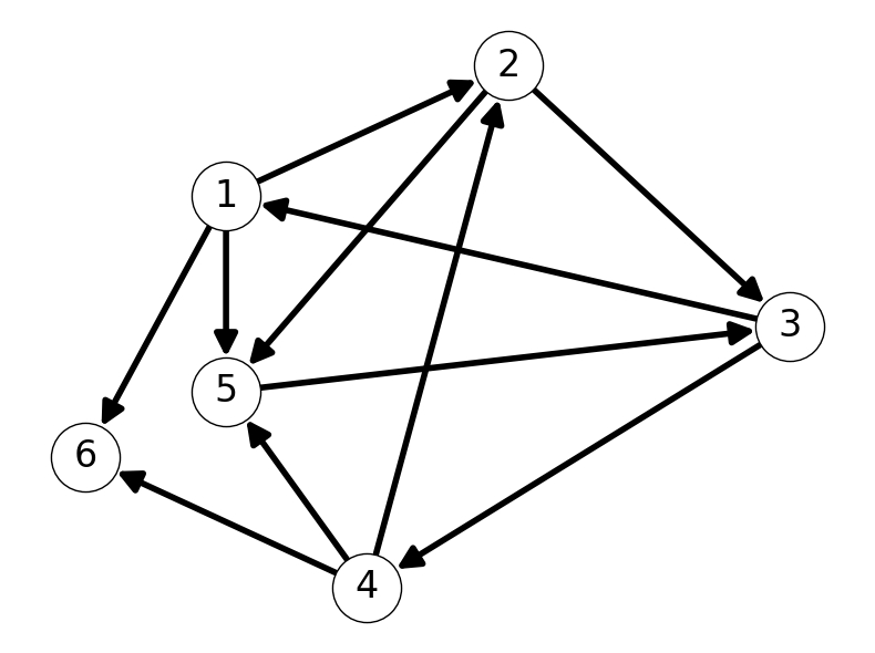
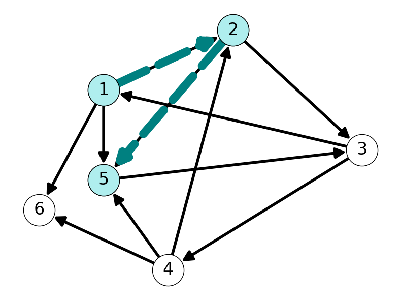
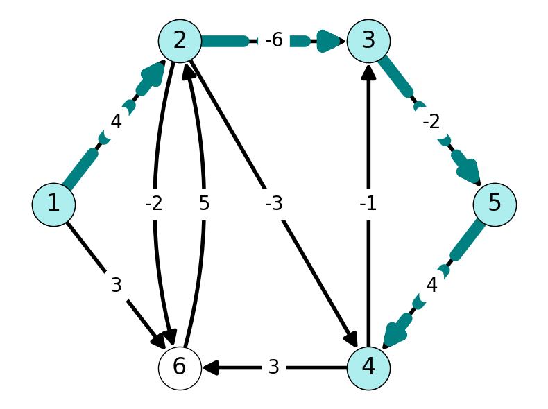
Example 5.4 Figure 5.4 gives the shortest \((1,t)\)-paths in the graph given in Figure 5.4 (a) for \(t = 2,3,4,5,6\).
5.2.2 Subpath Optimality
The following theorem characterizes a very useful properties of shortest paths: any subpath of a shortest path is itself a shortest path.
Theorem 5.3 Let \(P = (s,i_2), (i_2, i_3), \dots, (i_{k-1}, t)\) be a shortest \((s,t)\)-path.
Consider pair of nodes \(i_u, i_v\) visited by \(P\) with \(u < v\).
Then the subpath from \(i_u\) to \(i_v\) is a shortest \((i_u,i_v)\) path.
Proof. Suppose, on the contrary, that the subpath \(S\) from \(i_u\) to \(i_v\) in a shortest \((s,t)\)-path is not the shortest \((i_u, i_v)\)-path. In particular, suppose that \(T\) is the shortest \((i_u, i_v)\)-path.
We can construct another \((s,t)\)-path \(tilde P\) using \(P\) and \(T\). Indeed, let \(\tilde P = P \setminus S \cup T\) be the path obtained by removing \(S\) from \(P\) and adding \(T\). Then \(\tilde P\) is also a \((s,t)\)-path. The length of \(\tilde P\) is equal to \[ |P| - |S| + |T| < |P| - |S| + |S| = |P| \] since \(|T| < |S|\). This implies that \(\tilde P\) is shorter than \(P\); this is a contradiction. Therefore, \(S\) must be the shortest \((i_u, i_v)\)-path.
5.2.3 Shortest Paths of Fixed Length
Definition 5.4 For all \(i\in V\), we define \(f_k(i)\) as the length of a shortest \((s,i)\)-path containing at most k arcs,
We set \(f_k(i) = \infty\) if there is no \((s,i)\)-path with length at most \(k\).
Lemma 5.1 If \(k = n-1\), then \(f_{n-1}(i)\) is the length of a shortest \((s,i)\)-path (without restriction on the number of arcs).
Proof. We can ignore paths that aren’t simple. On the other hand, simple paths contain at most \(n\) nodes. Indeed, a simple path does not contain a loop and, hence, visits at most \(n\) nodes. Therefore, the shortest \((s,i)\)-path contains at most \(n-1\) arcs.
5.2.4 The Bellman-Ford Theorem
The following theorem is the basis for our algorithm for calculating shortest paths.
Theorem 5.4 \(f_k(i)\) can be computed recursively as \[ f_k(i) = \min \left\{ f_{k-1}(i), \; \min_{(j,i) \in \delta^-(i)} \Big\{ f_{k-1}(j) + \ell_{ji} \Big\} \right\}. \]
Proof. Assume that \(f_{k-1}(i)\) has been computed for all \(i \in V\setminus\{s\}\). The shortest \((s,i)\)-path with at most \(k\) arcs
is the shortest \((s,i)\)-path with at most \(k-1\) arcs; or
contains one more arc than the shortest \((s,i)\)-path with at most \(k-1\) arcs.
In the second case, we can decompose the shortest \((s,i)\)-path as:
shortest \((s,j)\)-path with \(k-1\) arcs for some node \(j\); and
arc \((j,i)\).
We choose node \(j\) so that \(j\) gives \[ \min_{(q,i) \in \delta^-(i)} f_{k-1}(q) + \ell_{qi}. \]
5.2.5 The Bellman-Ford Algorithm
5.2.5.1 Setup
Definition 5.5 Let \(P_k(i)\) be the predecessor of \(i\) in the shortest \((s,i)\)-path with at most \(k\) arcs found by the algorithm (so far).
We will maintain two tables:
One encoding \(f_k(i)\) for each \(i\) and \(k\);
The other encoding \(P_k(i)\) for all \(i\) and \(k\).
5.2.5.2 Updates
The algorithm calculates \(f_k(i)\) and \(P_k(i)\) for all \(i \in V\) recursively from \(k=1\) to \(k=n-1\).
We’ll update \(f_k(i)\) from \(f_{k-1}(i)\) by:
Initially setting \(f_k(i) = f_{k-1}(i)\);
Scanning all arcs \((j,i)\) in \(\delta^{-}(i)\) and update \(f_k(i)\) if necessary.
5.2.5.3 The Bellman-Ford Algorithm (Pseudocode)
f_0(s) = 0 and P_0(s) = ~
for i in V \{s}:
    f_0(i) = +inf and  P_0(i) = ~

# Calculate shortest paths of length k.
for k in {1, 2, ..., n-1}:

    # Update shortest si-path.
    for i in V:
        f_k(i) = f_{k-1}(i)
        P_k(i) = P_{k-1}(i)

        # Check each edge incident at i.
        for (j,i) in delta^{-}(i):
            # Update if length-k path is shorter than k-1.
            if f_{k-1}(j) + l_{ji} < f_k(i)
                f_k(i) = f_{k-1}(j) + l_{ji}
                P_k(i) = j
5.2.6 Example
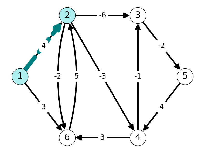
5.2.6.1 Iteration 1 (\(k=1\))
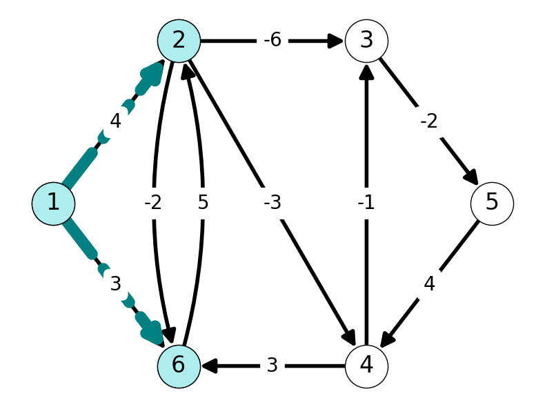
Note that nodes \(2\) and \(6\) are adjacent to \(1\). Thus, they are reachable from \(1\) by a path with length at most \(1\). The only paths from \(1\) to another node are the single arcs \((1,2)\) and \((1,6)\), of lengths \(4\) and \(3\) respectively. Figure 5.5 highlights these paths, and we update the tables Table 5.1 and Table 5.2 accordingly.
| 1 | 2 | 3 | 4 | 5 | 6 | |
|---|---|---|---|---|---|---|
| \(f_0\) | 0 | \(\infty\) | \(\infty\) | \(\infty\) | \(\infty\) | \(\infty\) |
| \(f_1\) | 0 | 4 | \(\infty\) | \(\infty\) | \(\infty\) | 3 |
| 1 | 2 | 3 | 4 | 5 | 6 | |
|---|---|---|---|---|---|---|
| \(P_0\) | \(\sim\) | \(\sim\) | \(\sim\) | \(\sim\) | \(\sim\) | \(\sim\) |
| \(P_1\) | \(\sim\) | 1 | \(\sim\) | \(\sim\) | \(\sim\) | 1 |
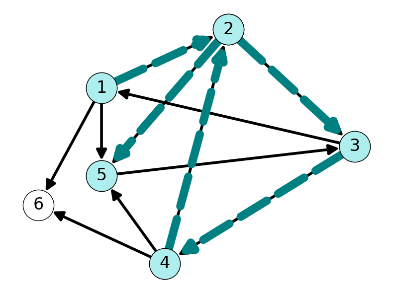
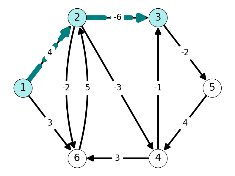
5.2.6.2 Iteration 2 (\(k=2\))
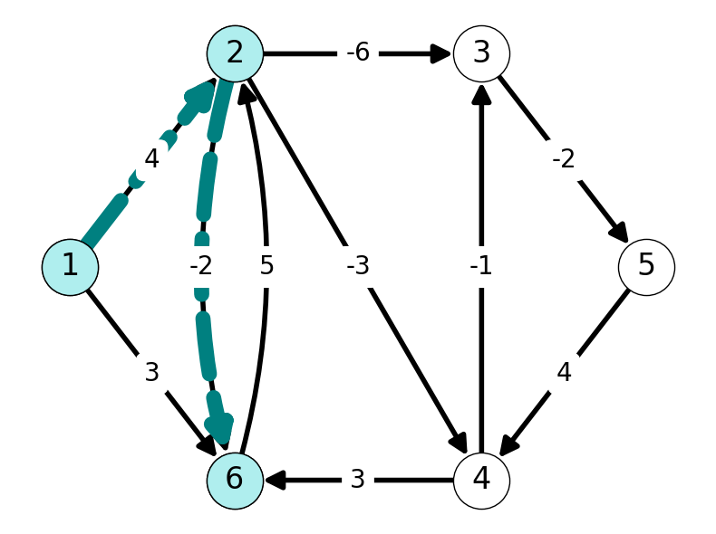
Nodes \(3\) and \(4\) can both be reached from \(1\) using a path of length \(2\) (with lengths \(-2\) and \(1\) respectively). Similarly, we have path \((1,2,6)\) of length \(2\): \[ \ell_{12} + \ell_{26} = f_1(2) + \ell_{26} = 4 - 2 = 2 < f_1(6) = 3. \]
This implies that the path \((1,2,6)\) is the shortest \((1,6)\)-path with at most \(2\) arcs. We update the shortest path and predecessor tables below.
| 1 | 2 | 3 | 4 | 5 | 6 | |
|---|---|---|---|---|---|---|
| \(f_0\) | 0 | \(\infty\) | \(\infty\) | \(\infty\) | \(\infty\) | \(\infty\) |
| \(f_1\) | 0 | 4 | \(\infty\) | \(\infty\) | \(\infty\) | 3 |
| \(f_2\) | 0 | 4 | -2 | 1 | \(\infty\) | 2 |
| 1 | 2 | 3 | 4 | 5 | 6 | |
|---|---|---|---|---|---|---|
| \(P_0\) | \(\sim\) | \(\sim\) | \(\sim\) | \(\sim\) | \(\sim\) | \(\sim\) |
| \(P_1\) | \(\sim\) | 1 | \(\sim\) | \(\sim\) | \(\sim\) | 1 |
| \(P_2\) | \(\sim\) | 1 | 2 | 2 | \(\sim\) | 2 |
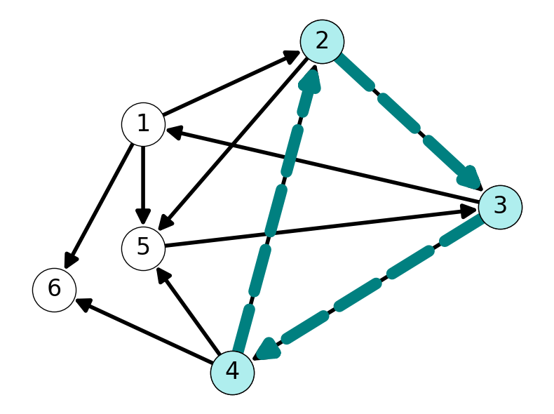
5.2.6.3 Iteration 3 (\(k=3\))
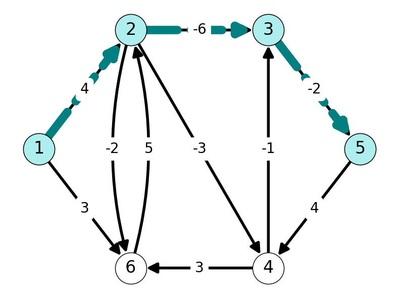
Node \(5\) is reachable from \(1\) by the path \((1,2,3,5)\) using \(3\) arcs; this path has length \(-4\). On the other hand, every other \((s,i)\)-path consisting of \(3\) arcs is longer than the shortest \((s,i)\)-path of length at most \(2\).

| 1 | 2 | 3 | 4 | 5 | 6 | |
|---|---|---|---|---|---|---|
| \(f_0\) | 0 | \(\infty\) | \(\infty\) | \(\infty\) | \(\infty\) | \(\infty\) |
| \(f_1\) | 0 | 4 | \(\infty\) | \(\infty\) | \(\infty\) | 3 |
| \(f_2\) | 0 | 4 | -2 | 1 | \(\infty\) | 2 |
| \(f_3\) | 0 | 4 | -2 | 1 | -4 | 2 |
| 1 | 2 | 3 | 4 | 5 | 6 | |
|---|---|---|---|---|---|---|
| \(P_0\) | \(\sim\) | \(\sim\) | \(\sim\) | \(\sim\) | \(\sim\) | \(\sim\) |
| \(P_1\) | \(\sim\) | 1 | \(\sim\) | \(\sim\) | \(\sim\) | 1 |
| \(P_2\) | \(\sim\) | 1 | 2 | 2 | \(\sim\) | 2 |
| \(P_3\) | \(\sim\) | 1 | 2 | 2 | 3 | 2 |
5.2.6.4 Iteration 4 (\(k=4\))
Note that we have the \((1,4)\)-path \((1,2,3,5,4)\) containing \(k=4\) arcs. This path has length \[ f_3(5) + \ell_{54} = -4 + 4 = 0 < f_3(4) = 1 = f_2(4). \] We set \(f_4(4) = 0\) and \(P_4(4) = 5\).
After checking all other paths containing \(k=4\) arcs, we do not change the list of shortest paths.

| 1 | 2 | 3 | 4 | 5 | 6 | |
|---|---|---|---|---|---|---|
| \(f_0\) | 0 | \(\infty\) | \(\infty\) | \(\infty\) | \(\infty\) | \(\infty\) |
| \(f_1\) | 0 | 4 | \(\infty\) | \(\infty\) | \(\infty\) | 3 |
| \(f_2\) | 0 | 4 | -2 | 1 | \(\infty\) | 2 |
| \(f_3\) | 0 | 4 | -2 | 1 | -4 | 2 |
| \(f_4\) | 0 | 4 | -2 | 0 | -4 | 2 |
| 1 | 2 | 3 | 4 | 5 | 6 | |
|---|---|---|---|---|---|---|
| \(P_0\) | 0 | \(\sim\) | \(\sim\) | \(\sim\) | \(\sim\) | \(\sim\) |
| \(P_0\) | \(\sim\) | \(\sim\) | \(\sim\) | \(\sim\) | \(\sim\) | \(\sim\) |
| \(P_1\) | \(\sim\) | 1 | \(\sim\) | \(\sim\) | \(\sim\) | 1 |
| \(P_2\) | \(\sim\) | 1 | 2 | 2 | \(\sim\) | 2 |
| \(P_3\) | \(\sim\) | 1 | 2 | 2 | 3 | 2 |
| \(P_4\) | \(\sim\) | 1 | 2 | 5 | 3 | 2 |
5.2.6.5 Termination
The shortest path using at most \(4\) arcs are also shortest paths using at most \(5\) arcs for this graph. Since \(k=5 = n-1\), we have found the shortest paths of any length by @lem.
5.2.7 Complexity of the Bellman-Ford Algorithm
Let’s analyses how many operations are needed by the Bellman-Ford Algorithm.
f_0(s) = 0 and P_0(s) = ~
for i in V \{s}:
    f_0(i) = +inf and  P_0(i) = ~

# Calculate shortest paths of length k.
for k in {1, 2, ..., n-1}:

    # Update shortest si-path.
    for i in V:
        f_k(i) = f_{k-1}(i)
        P_k(i) = P_{k-1}(i)

        # Check each edge incident at i.
        for (j,i) \in delta^{-}(i):
            # Update if length-k path is shorter than k-1.
            if f_{k-1}(j) + l_{ji} < f_k(i)
                f_k(i) = f_{k-1}(j) + l_{ji}
                P_k(i) = j
Initiailization (Lines 1-3) requires \(O(n)\) elementary operations.
The loop from Line 9 to Line 18 is repeated for each \(i \in V\) (\(O(n)\) times) and consists of the following steps for each \(i\):
Initializing \(f_k(i) = f_{k-1}(i)\) and \(P_k(i) = P_{k-1}(i)\) (requires \(O(1)\) operations).
Checking if each arc \((j,i)\) with tail \(i\) yields a shorter path with \(k\) arcs:
Comparing \(f_{k-1}(j) + \ell_{ji}\) with \(f_k(i)\) requires \(O(1)\) operations for each \(j\).
We have \(|\delta^-(i)| = O(n)\) of these arcs.
It follows that the loop from Lines 9–18 requires \[ O(n) \Big( O(1) + O(n) \Big) = O(n^2) \] for each \(k \in \{1,2,\dots, n-1\}\). Taking the total over all \(k\), the Bellman-Ford Algorithm requires \(O(n^3)\) elementary operations.
5.2.7.1 Complexity in Terms of Arcs
Each arc \((j,i) \in A\) is considered exactly once for each \(k \in \{1,2,\dots, n-1\}\) in the loop from Lines 9–18. This implies that the steps of this loop require \(O(|A| + n) = O(m + n)\) elementary operations. This implies that the total complexity of the Bellman-Ford Algorithm require \[ O(nm + n^2) \] elementary operations, which is much smaller than \(O(n^3)\) if \(m << n^2\).
5.2.8 Detecting Negative Length Cycles
Recall: SPP-U (and SSPP-U) are unbounded if the graph contains a negative length cycle. Indeed, we can endlessly apply rounds of update operations and reduce the shortest path lengths \(f_k(i)\) indefinitely.
We can detect whether the problem is unbounded by running one more iteration of the algorithm beyond iteration \(k = n-1\).
If the graph contains a negative-length cycle then an update will take place.
This indicates the problem is unbounded and we can stop the algorithm.
5.2.8.1 Example
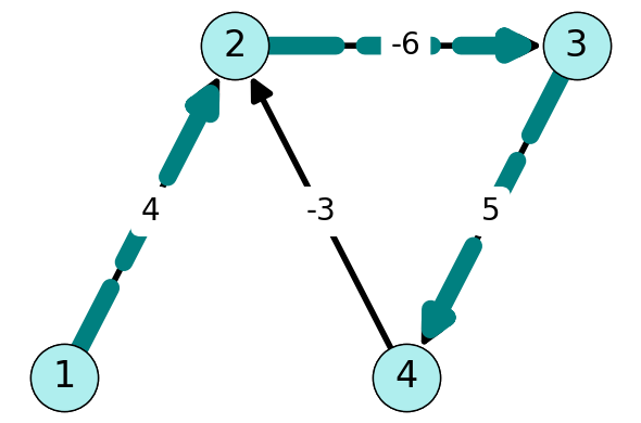
Consider the graph given in Figure 5.9. This graph has cycle \(C = (2,3,4,2)\) with length \(-4 < 0\).
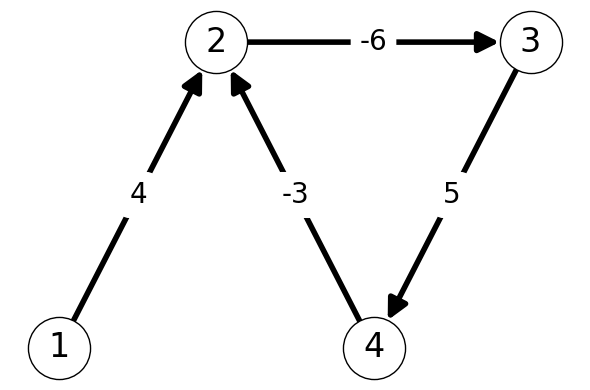
Let’s apply the Bellman-Ford algorithm to find the shortest \((1,t)\)-paths in this graph.
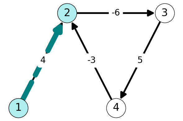
5.2.8.1.1 Iteration 1 (\(k=1\))
The only node adjacent to \(1\) is \(2\). Thus, the
| 1 | 2 | 3 | 4 | |
|---|---|---|---|---|
| \(f_0(i)\) | 0 | \(\infty\) | \(\infty\) | \(\infty\) |
| \(f_1(i)\) | 0 | 4 | \(\infty\) | \(\infty\) |
| 1 | 2 | 3 | 4 | |
|---|---|---|---|---|
| \(P_0(i)\) | \(\sim\) | \(\sim\) | \(\sim\) | \(\sim\) |
| \(P_1(i)\) | \(\sim\) | 1 | \(\sim\) | \(\sim\) |
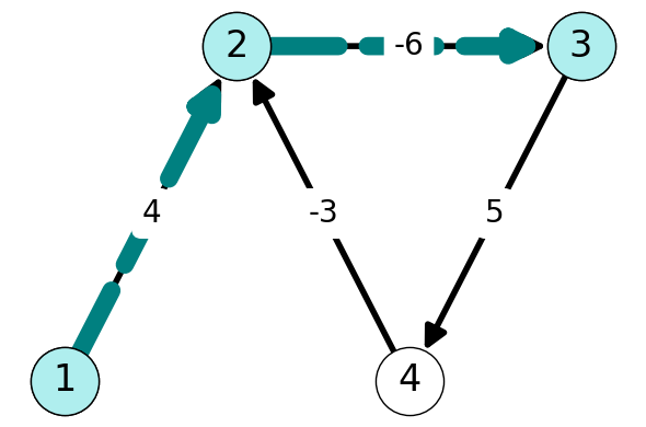
5.2.8.1.2 Iteration 2 (\(k=2\))
Next, we can reach \(3\) from \(1\) via a path consisting of \(2\) arcs. This path has length \(-2\).
| 1 | 2 | 3 | 4 | |
|---|---|---|---|---|
| \(f_0(i)\) | 0 | \(\infty\) | \(\infty\) | \(\infty\) |
| \(f_1(i)\) | 0 | 4 | \(\infty\) | \(\infty\) |
| \(f_2(i)\) | 0 | 4 | -2 | \(\infty\) |
| 1 | 2 | 3 | 4 | |
|---|---|---|---|---|
| \(P_0(i)\) | \(\sim\) | \(\sim\) | \(\sim\) | \(\sim\) |
| \(P_1(i)\) | \(\sim\) | 1 | \(\sim\) | \(\sim\) |
| \(P_2(i)\) | \(\sim\) | 1 | 2 | \(\sim\) |
5.2.8.1.3 Iteration 3 (\(k=3\))
Node \(4\) is the only node that is reachable from \(1\) by a path containing \(3\) arcs; the path \((1,2,3,4)\) has length \(3\).
| 1 | 2 | 3 | 4 | |
|---|---|---|---|---|
| \(f_0(i)\) | 0 | \(\infty\) | \(\infty\) | \(\infty\) |
| \(f_1(i)\) | 0 | 4 | \(\infty\) | \(\infty\) |
| \(f_2(i)\) | 0 | 4 | -2 | \(\infty\) |
| \(f_3(i)\) | 0 | 4 | -2 | 3 |
| 1 | 2 | 3 | 4 | |
|---|---|---|---|---|
| \(P_0(i)\) | \(\sim\) | \(\sim\) | \(\sim\) | \(\sim\) |
| \(P_1(i)\) | \(\sim\) | 1 | \(\sim\) | \(\sim\) |
| \(P_2(i)\) | \(\sim\) | 1 | 2 | \(\sim\) |
| \(P_3(i)\) | \(\sim\) | 1 | 2 | 3 |
5.2.8.1.4 Iteration 4 (\(k=4\))
Let’s try one more iteration!
Note that \[ f_3(4) + \ell_{42} = 3 - 3 = 0 < f_2(2). \]
| 1 | 2 | 3 | 4 | |
|---|---|---|---|---|
| \(f_0(i)\) | 0 | \(\infty\) | \(\infty\) | \(\infty\) |
| \(f_1(i)\) | 0 | 4 | \(\infty\) | \(\infty\) |
| \(f_2(i)\) | 0 | 4 | -2 | \(\infty\) |
| \(f_3(i)\) | 0 | 4 | -2 | 3 |
| \(f_4(i)\) | 0 | 0 | -2 | 3 |
| 1 | 2 | 3 | 4 | |
|---|---|---|---|---|
| \(P_0(i)\) | \(\sim\) | \(\sim\) | \(\sim\) | \(\sim\) |
| \(P_1(i)\) | \(\sim\) | 1 | \(\sim\) | \(\sim\) |
| \(P_2(i)\) | \(\sim\) | 1 | 2 | \(\sim\) |
| \(P_3(i)\) | \(\sim\) | 1 | 2 | 3 |
| \(P_4(i)\) | \(\sim\) | 4 | 2 | 3 |
This implies that the path \((1,2,3,4,2)\) with \(5\) arcs has smaller total length than the path \((1,2)\). This contradicts Lemma 5.1 and, hence, implies that the shortest path problem is unbounded for this graph. Indeed, further iterations will lead further decrease in \(f_k(i)\) for \(i\) in the negative length cycle \((2,3,4,2)\). We can stop the Bellman-Ford Algorithm after \(k=n\) iterations and declare the problem instance unbounded.