6 Minimum Cost Spanning Trees

6.1 Preliminaries

6.1.1 Subgraphs

Definition 6.1 Let $G = (V,E)$ be an undirected graph.

We call $G_S = (V_S, E_S)$ a subgraph of $G$ if

$G_S$ is a graph;
$V_S \subseteq V$ and $E_S \subseteq E$.

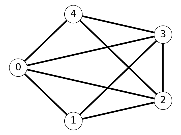
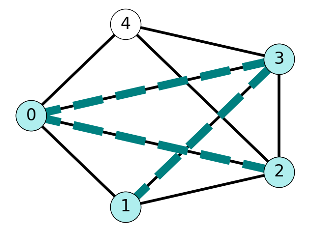
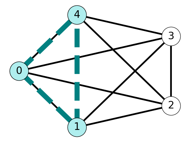
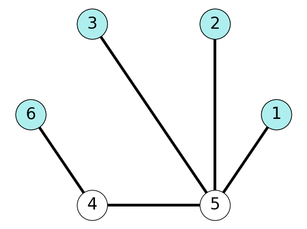
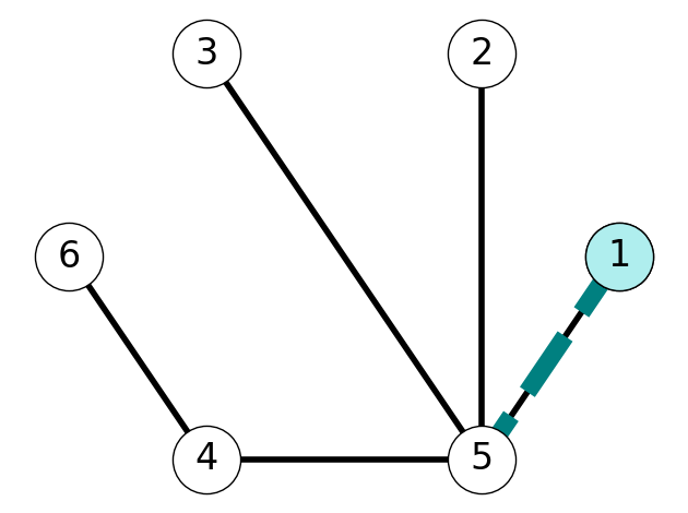
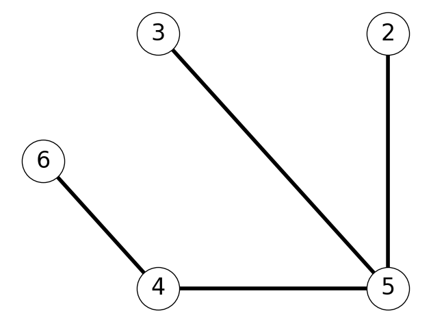
Example 6.1 Consider the graph $G = (V,E)$ given in Figure 6.2 (a). The graph given in Figure 6.2 (b) is a subgraph of $G$. However, the graph given in Figure 6.2 (c) is not a subgraph of $G$ since $\{1,4\} \notin E$.

6.1.2 Trees

Definition 6.2 Let $G = (V,E)$ be an undirected graph.

The subgraph $G_T = (V_T, E_T)$ is a tree if

$G_T$ is a connected;
$G_T$ is acyclic, i.e., contains no cycles.

A tree $G_T$ is a spanning tree if $V_T = V$ ($G_T$ spans/reaches all nodes in $V$).

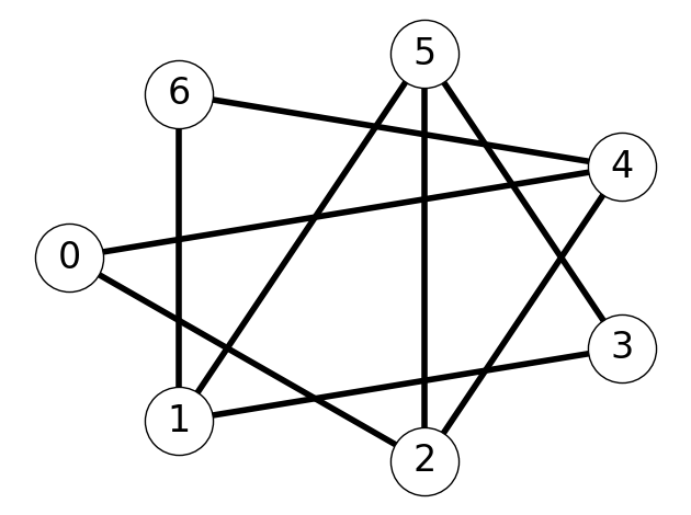
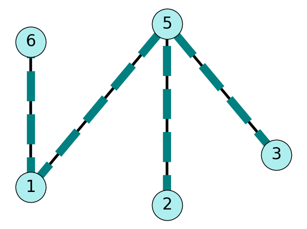
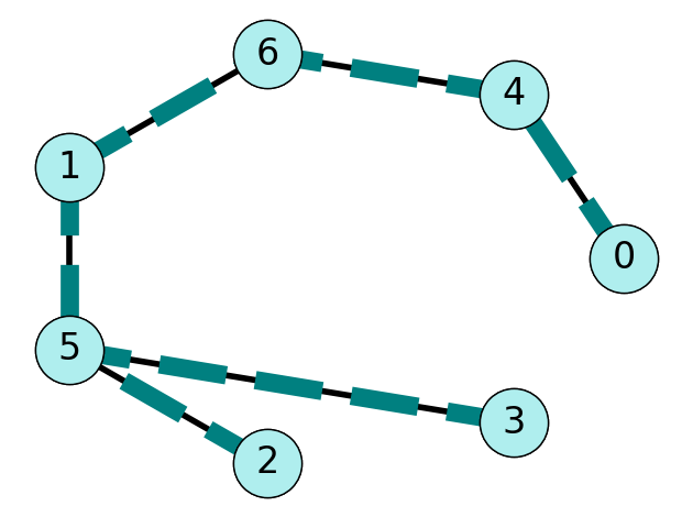
Example 6.2 Consider the graph $G = (V,E)$ given in Figure 6.2 (a). The subgraph given in Figure 6.2 (b) is a connected and acyclic; therefore, it is a tree. On the otherhand, the subgraph given in Figure 6.2 (c) is a tree and has node set $V$; therefore, it is a spanning tree.

6.1.3 Motivating Example

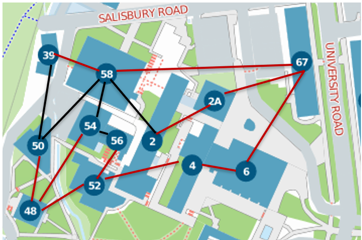
We want to build a new high-speed network at the University:

should connect all buildings; while
costing as little as possible.

We can model this problem as that of finding a minimum cost spanning tree.

Consider the graph $G$ with:

Buildings as vertices;
Potential connections as edges.

We want to find a connected, acyclic subgraph to minimize cost while ensuring all buildings are connected. Such a tree is highlighted in red in Figure 6.3.

Figure 6.3: Campus map with minimum spanning tree

6.1.4 The Minimum Cost Spanning Tree (MST) Problem

Definition 6.3 Given an undirected graph $G = (V,E)$ and cost function $c: E\mapsto \mathbf{R}$.

The minimum cost spanning tree problem aims to find a spanning tree $G_T = (V_T, E_T)$ of minimum total cost: \[\min~ c(E_T) = \sum_{e \in E_T} c_e.\]

Theorem 6.1 (Cayley – 1889) A complete undirected graph with $n$ nodes contains $n^{n-2}$ spanning trees.

Noncomplete graphs contain fewer spanning trees, but the number is still exponentially large in $n$. This implies that we cannot solve MST using complete enumeration for even small graphs.

6.1.5 Leaves

Definition 6.4 The nodes of a graph with degree 1 are called leaves.

Theorem 6.2 A tree contains at least one leaf.

Proof. Suppose, on the contrary, that tree $T$ does not contain a leaf. Then every node in $T$ has degree at least $2$. This implies that $T$ has a cycle; a contradiction.

Figure 6.4: A tree with leaves ${1, 2, 3, 6}

6.1.6 The Number of Edges of A Tree

Theorem 6.3 A tree $G_T$ with $n$ nodes has $m = n-1$ edges.

Proof. We’ll prove Theorem 6.3 by induction.

As a base case, consider $n=1$. This tree consists of a single node and $0 = n-1$ edges.

Now suppose that every tree with $k$ nodes has $n-1$ edges. Consider tree $T$ with $k+1$ nodes. We want to show that $T$ has $k$ edges.

To do so, note that $T$ contains at least one leaf by Theorem 6.2. Without loss of generality, let’s assume that node $1$ is a leaf; if not, we can relabel vertices so that $1$ is a leaf. Let’s remove leaf $1$ and its incident edge (there is only one such edge because $1$ has degree-$1$).

After deleting this node and edge, we have a connected, acyclic graph with $k$ nodes. By the inductive hypothesis, this tree has $k-1$ edges. Since we deleted $1$ node and $1$ edge, we can conclude that $T$ had $k$ edges. This completes the proof.

6.1.7 The Swap Property

Lemma 6.1 Given tree $G_T = (V_T, E_T)$, removing an edge $e \in E_T$ creates two subtrees.

6.1.8 Swapping Edges Within a Cut

Lemma 6.2 Let $S$ be the vertex set of one of the two subtrees.

For every edge $f \in \delta(S)$ other than $e$, the set \[ E_T' := E_T \cup \{f\} \setminus \{e\} \] is the edge set of a tree spanning the same set of nodes.

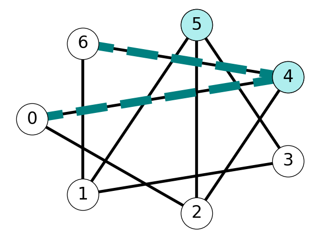
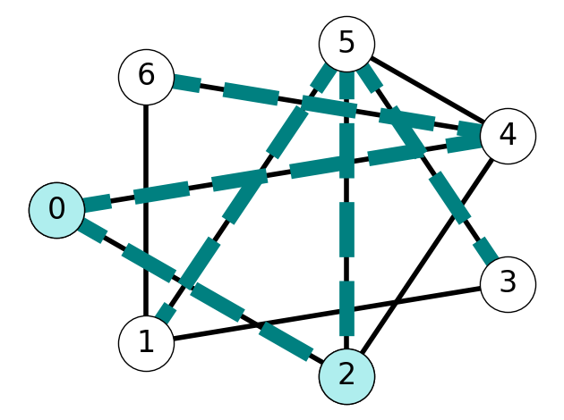
Example 6.3 Consider the graph $G$ with tree $T$ given by Figure 6.7 (a). The example in Figure 6.6 illustrates that we obtain two subtrees after removing edge $e=45$.

The set $S = \{1,2,3, 5\}$ is the vertex set of one of these trees. The cut induced by $S$ is \[ \delta(S) = \{02, 16, 24\}. \] Lemma 6.2 implies that exchanging $02$ with $45$ yields a new tree $\tilde{T}$ with edge set \[ E_{\tilde T} = E_T \setminus \{4,5\} \cup \{0,2\} = \{15, 25, 35, 46, 02\}. \] See Figure 6.7 for an illustration of this process.

6.2 The Jarnik-Prim-Dijkstra Algorithm

6.2.1 Jarnik’s Theorem

Theorem 6.4 (Jarnik’s Theorem)

Let $F$ be the edge set of a tree strictly contained in an MST.
Let $S\subseteq V$ be the set of nodes it spans.

For every edge $e \in \delta(S)$:

$F \cup \{e\}$ is part of a MST if and only if $e$ has minimum cost in $\delta(S)$.

Proof. We start by proving the “only if” part. Let’s suppose that $F \cup \{e\}$ is part of a MST. We want to show that $e$ has minimum cost in $\delta(S)$ in this case. We’ll use a proof by contradiction. Let’s assume that there is $f\in \delta(S)$ with $c_f < c_e$.

Let $T = (V, E_T)$ be a minimum spanning tree such that $F \subseteq E_T$ and $F \cup \{e\} \subseteq E_T$. By the Swap Property (Lemma 6.1) the subgraph \[ \tilde T = (V, E_T\setminus\{e\} \cup \{f\}) \] is also a spanning tree. Moreover, the cost of $\tilde T$ satisfies \[ c(\tilde T) = c(T) - c_e + c_f < c(T) \] since $c_e > c_f$.

This implies that $T$ is not a minimum cost spanning tree; a contradiction. Therefore, we can conclude that if $F \cup \{e\}$ is part of a minimum spanning tree then $c_e \le c_f$ for all $f \in \delta(S)$.

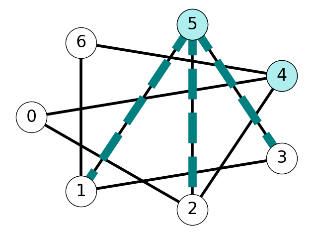
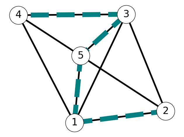
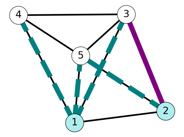
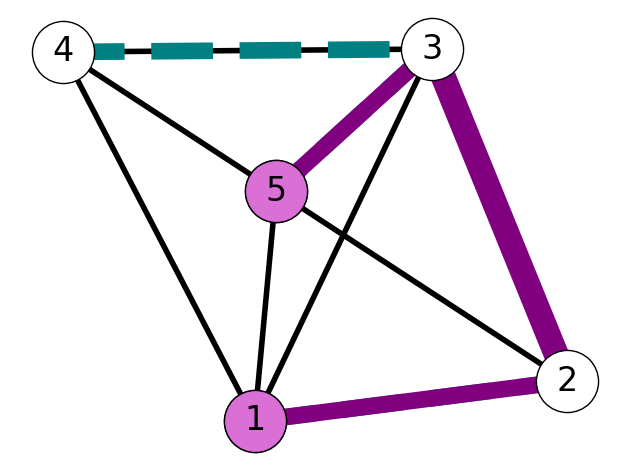
This is illustrated in Figure 6.8. Consider the spanning tree $T$ given in Figure 6.8 (a) and the edge set $F = \{12\} \subseteq E_T$; here, $S = \{1,2\}$. Note that $e = 15$ is in the both $E_T$ and $\delta(S)$, while $f=23$ belongs to $\delta(S)$, but not $E_T$. The swap property implies that we can obtain a spanning tree $\tilde T$ by exchanging the edges $e$ and $f$. If $c_f < c_e$ then $\tilde T$ is a spanning tree with strictly lower cost than $T$.

We next prove the “if” part. That is, we prove that if $e$ has minimum cost in $\delta(S)$ then $F \cup \{e\}$ is part of a minimum spanning tree. To do so, suppose that $c_e \le c_f$ for all $f \in \delta(S)$. We want to show that $F \cup \{e\}$ is part of a MST.

We consider two cases. First, suppose that $e \in E_T$, where $T$ is the MST containing $f$. This immediately implies that $e$ belongs to a MST and we’re done.

Next, suppose that $e \notin E_T$. Specifically, let $e = uv$ for nodes $u, v \in V$ such that $e \notin E_T$ and $e \in \delta(S)$; we assume that $u \in S$ and $v \in V \setminus S$.

Let $P$ be the $(u,v)$-path joining the end points of $e$ belonging to $T$. Such a path always exists because $T$ is a spanning tree. Since $P$ starts in $S$ at $u$ and ends in $V\setminus S$ at $v$ there is at least one edge $f$ in both $P$ and $\delta(S)$, i.e., there is edge $f \in P \cap \delta(S)$.

By the swap property, the subgraph \[ T' = (V, E_T \setminus \{f\} \cup \{e\}) \] is a spanning tree. Moreover, \[ c(T) \ge c(T') = c(T) - c_f + c_e \le c(T) \] since $T$ is a minimum spanning tree and $c_e \le c_f$. This is only possible if $c_e = c_f$ and $T'$ is also a minimum spanning tree.

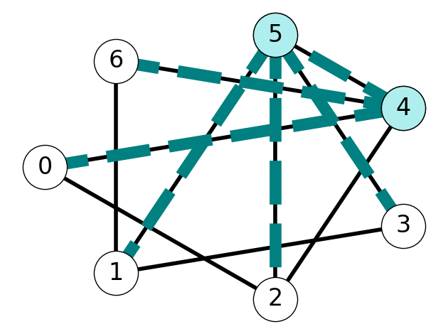
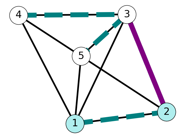
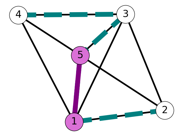
To illustrate this phenomena, consider the edge $e = 15$ in Figure 6.9. This edge is not included in the minimum spanning tree $T$. However, there is a path $P = (1,2,3,5)$ in $T$ containing the edge $f = 23 \in \delta(\{1,2\})$. Applying the swap property and the assumption the $c_e \le c_f$ shows that $T'$ is also a minimum cost spanning tree.

(a) Minimum spanning tree $T$ not including $e = 15$.

6.2.2 The Jarnik-Prim-Dijkstra (JPD) Algorithm

Theorem 6.4 suggests the following algorithm for identifying a minimum cost spanning tree in a given graph.

Initialize E_T = {} and S = {1}.

While |E_T| < n-1:

    Choose e = {v,w} in delta(S) of minimum cost c_e.  

    Update E_T = E_T + {e} 

    Update S = S + {w}.

6.2.2.1 Complexity of the JPD Algorithm

For each step of the while loop, choosing $e$ in Line 5$ costs $O(m)$ operations to search over the set of edges in $\delta(S)$. The loop is repeated $O(n)$ times, so the total complexity is $O(mn)$ elementary operations. This may be as large as $O(n^3)$ when the graph is very dense of as small as $O(n^2)$ when the graph is very sparse but still connected.

6.2.3 Example: MST for Flight Routing

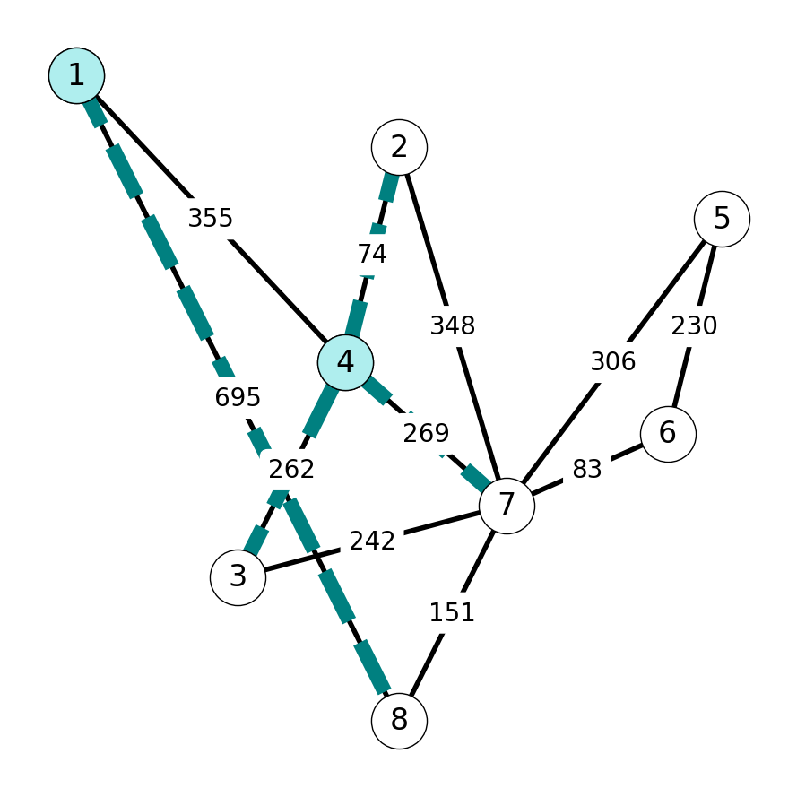
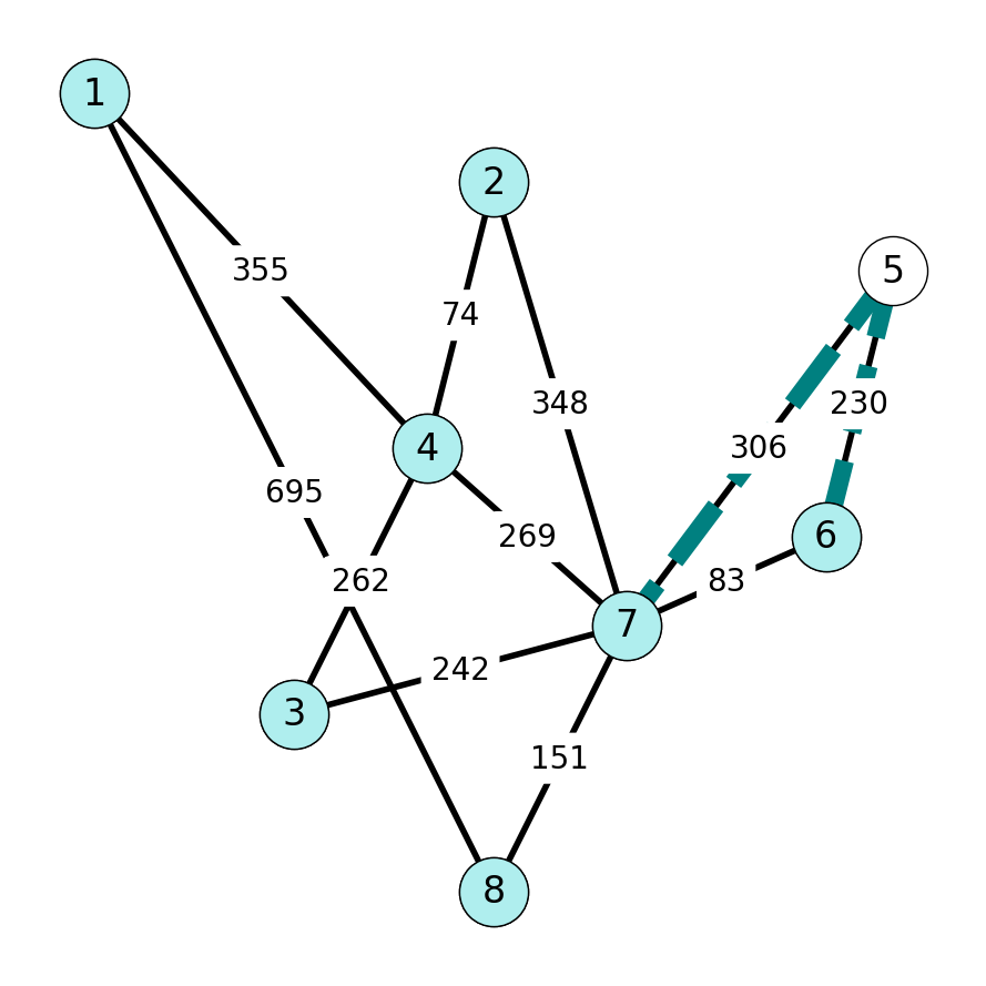
The following graph $G = (V, E)$ gives available/potential flight routes between 8 cities, with distances in miles. The MST of $G$ gives an airline a means of servicing each city while minimizing travel distance and fuel costs.

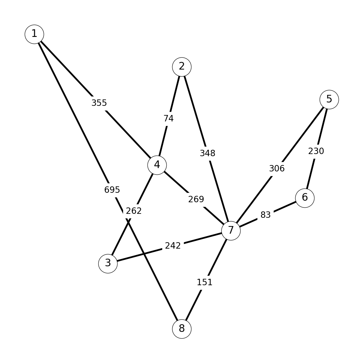
Let’s apply the Jarnik-Prim-Dijsktra Algorithm to find the minimum cost spanning tree in $G$.

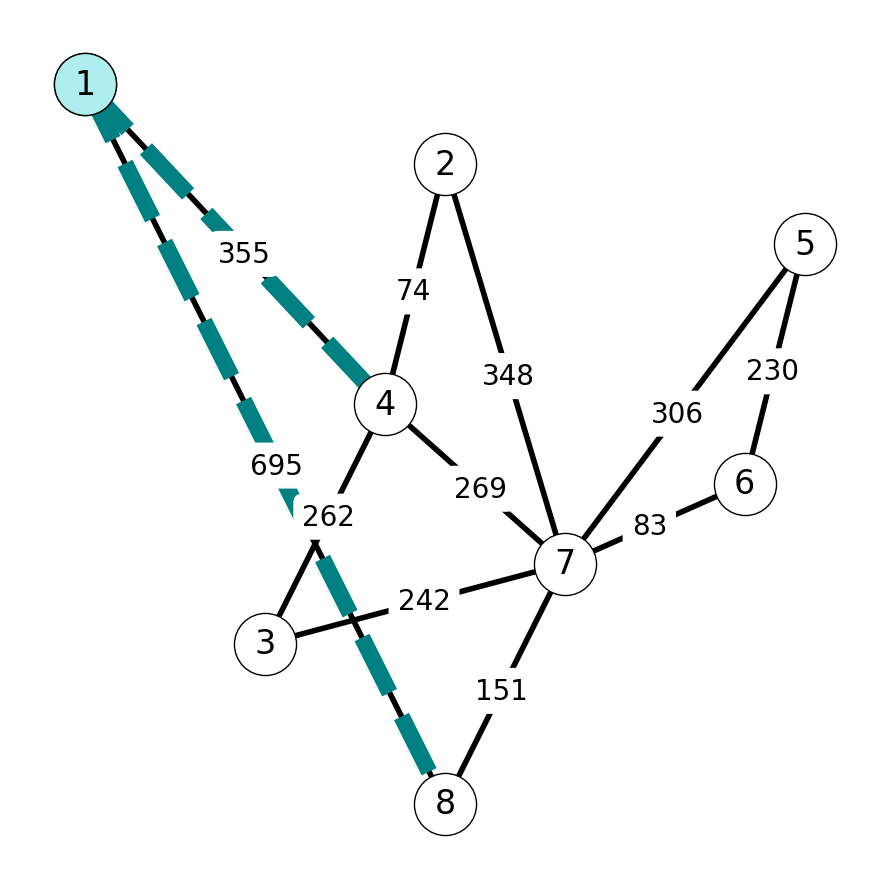
Step 1

We start with $S = \{1\}$, which induces the cut $\delta(S) = \{14, 18\}$. Since \[ c_{14} = 355 < 695 = c_{18}, \] we add $14$ to $E_T$ and add $\{4\}$ to $S$.

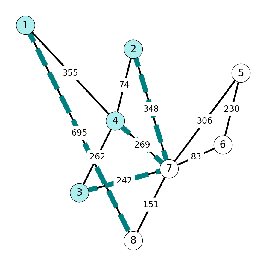
Step 2

Next, $\delta(S) = \{18, 24, 34, 74\}$. We add $2$ to $S$ and $24$ to $E_T$ because $c_{24} = 74$ is the minimum cost edge in $\delta(S)$.

Step 3

Next, $c_{34} = 262$ has minimum cost among edges in $\delta(S) = \{18, 34, 47, 27\}$. We add $34$ to $E_T$ and $3$ to $S$.

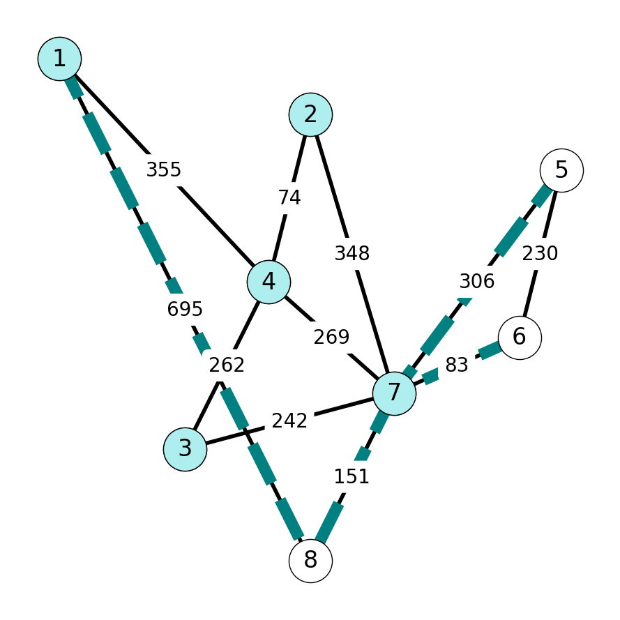
Step 4

We next add $37$ to $E_T$ and $7$ to $S$ because $c_{37} = 242$ has minimum cost among edges in $\delta(S) = \{37, 47, 27, 18\}$.

Step 5

We next add $67$ to $E_T$ and $6$ to $S$ because $c_{67} = 83$ has minimum cost among edges in $\delta(S) = \{18, 75, 76, 78\}$.

Step 6

Next, $c_{78} = 151$ is minimum cost among edges in $\delta(S) = \{18, 56, 57, 78\}$. Add $8$ to $S$ and $78$ to $E_T$.

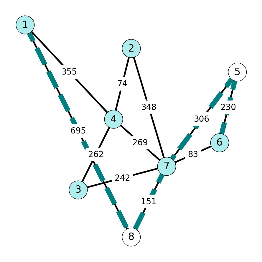
Step 7

Finally, $\delta(S) = \{56, 57\}$. We have \[ c_{56} = 230 < 306 = c_{57}, \] so we add $56$ to $E_T$, $5$ to $S$.

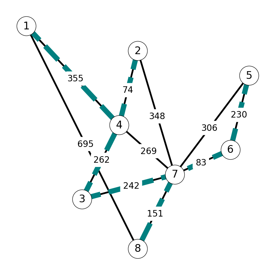
Termination

Note that $S = \{V\}$ and $E_T$ contains $n-1=7$ edges. This implies that we have constructed the minimum spanning tree $T$.

Figure 6.18: Minimum spanning tree identified by the JPD Algorithm

6.3 Improving the JPD Algorithm

6.3.1 Inefficiency of Searching over Edges

Problem: The algorithm scans many edges that will never be selected.

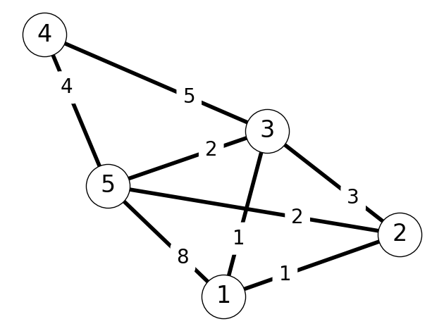
To see why this may be the the case, consider the set $S = \{1, 3, 5\}$ in the graph given in Figure 6.19.

Figure 6.19: Graph $G$ with $S = \{1,3,5\}$

For $S = \{1,3,5\}$, we have $\delta(S) = \{21, 23, 25, 41, 45 \}$. The JPD Algorithm will add edge $45$ with minimum cost to $E_T$, but will consider every edge in $G$. However, we know that the only candidates to be added to $S$ are Nodes $2$ and $4$. Since $23$ and $45$ are the minimum cost edges incident with $2$ and $4$ respectively, we really only need to consider these two edges as candidates for $E_T$.

This example implies that if we knew which edge incident with each node has minimum cost, then we can search among nodes, not edges. Since we usually have far fewer nodes than edges, this can lead to substantial improvement in computational cost.

6.3.2 Node Labels

To facilitate this, let’s introduce two labels for each node $j \in V \setminus S$:

$C(j) := \min_{i \in S}~c_{ij}$ (minimum cost of edge connecting $S$ to $j$);
$P(j) := \text{argmin}_{i \in S}~c_{ij}$ (endpoint in $S$ of this minimum cost edge).

Example 6.4 For the graph given in Figure 6.19, we have \[ \begin{aligned} C(2) &= 4, & C(4) &= 2 \\ P(2) &= 3, & P(3) &= 5. \end{aligned} \]

If we have $C$ and $P$, choosing the vertex $w$ to add to minimum spanning tree should only require $O(n)$ EOs to compare the values of $C$ for the vertices in $V\setminus S$.

Further, we must update $C$ and $P$ whenever $S$ is updated. To do so, we search the star of $w$, which requires $O(n)$ EOs.

The total complexity is $O(n)$ per iteration and $O(n^2)$ total. This can be much smaller than $O(mn)$!!

6.3.3 Better Algorithm – Pseudocode

This suggests the following algorithm.

Let S = {1}, E_T = {}, C(1) = 0.

% Initialize costs.
For j in V - {1}
    Let C(j) = c_{1j} and P(j) = 1
    (assume c_{1j} = inf if 1j not in E).

While |E_T| < n-1

    Find w in V \ S minimizing C(w). 

    Let S = S + {w} and E_T = E_T + {P(w), w}.  

    % Update costs
    For j in V \ S such that wj in delta(w)

        If c_{wj} < C(j): 
            Update C(j) = c_{wj} and P(j) = w.

6.3.4 Another Example

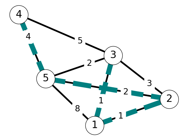
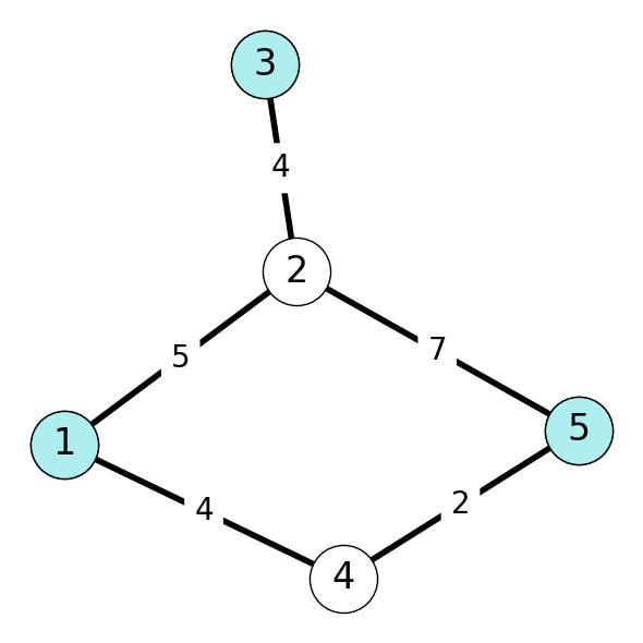
To illustrate the application of the revised algorithm, let’s consider the graph $G$ given in Figure 6.20.

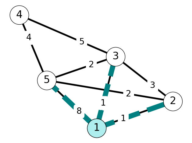
Step 1

Initially, we have $S = \{1\}$. Note that \[ \begin{aligned} C(2) &= c_{12} = 1 \\ C(3) &= c_{13} = 1 \\ C(4) &= + \infty \\ C(5) &= c_{15} = 8. \end{aligned} \] We choose $w=2$. We add $2$ to $S$ and $12$ to $E_T$. Note that we could also choose to add $3$ to $S$ and $13$ to $E_T$ since $c_{12} = c_{13} = 1$.

It remains to update $C$ and $P$. Note that \[ \begin{aligned} C(3) &= c_{13} = 1 < c_{23} = c_{w3} \\ c_{w5} &=c_{25} = 2 < C(5). \end{aligned} \] Thus, we set $C(5) = 2$ and $P(5) = 2$ and leave $C(3)$, $P(3)$ unchanged.

Figure 6.21: Step 1 of the revised JPD algorithm

Predecessor and value of minimum cost $(1,v)$-path found so far.
v	C(v)	P(v)
2	1	1
3	1	1
5	2	2

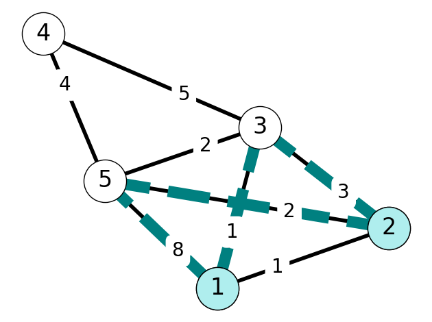
Step 2

We have $S = \{1,2\}$. Nodes $3$ and $5$ are adjacent to $1$ and $2$. Since \[ C(3) = 1 < 2 = C(5), \] we add $3$ to $S$; since $P(3)=1$, we add $13$ to $E_T$. Finally, we update \[ C(4) = 5, P(4) = 3 \] since $4$ is adjacent to $3$; $C(5)$ and $P(5)$ are unchanged.

Predecessor and value of minimum cost $(1,v)$-path found after two steps of revised JPD algorithm.
v	C(v)	P(v)
2	1	1
3	1	1
4	5	3
5	2	2

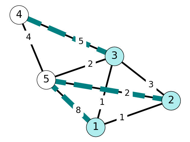
Step 3

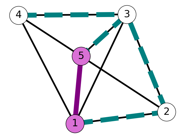
Since $C(5) < C(4)$, we add $5$ to $S$ and $25$ to $E_T$. Note that \[ c_{45} = 4 < C(4) = 5, \] we set $C(4) = 4$ and $P(4) = 5$.

Predecessor and value of minimum cost $(1,v)$-path found after three steps of revised JPD algorithm.
v	C(v)	P(v)
2	1	1
3	1	1
4	5	3
5	2	2

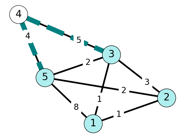
Step 4

The only edge left to add $E_T$ is $54$.

Predecessor and value of minimum cost $(1,v)$-path found after four steps of revised JPD algorithm.
v	C(v)	P(v)
2	1	1
3	1	1
4	4	5
5	2	2

This gives the minimum cost spanning tree $T$ found in Figure 6.25.

Figure 6.25: Mininum spanning tree in $G$