7 Network Flows
7.1 Model Formulation
7.1.1 Motivation
We want to figure out the maximum amount of some commodity can be transported from a certain node \(s\) to another point \(t\) of a network.
This can take the form of any of the following (among many other examples):
- Oil, water, really any fluid in pipeline network;
- Vehicle traffic in a roadway network;
- Information in a communication network;
- Spread of disease in pandemic models.
7.1.2 Standard Constraints
Regardless of physical application/interpretation of the network, we have the following standard collection of constraints.
7.1.2.1 Capacity constraints
Each pipe cannot carry more than its capacity.
Let \(x_{ij}\) denote the amount of commodity carried from \(i\) to \(j\) and let \(k_{ij}\) denote the capacity of the pipe from \(i\) to \(j\).
Then we must have \[ 0 \le x_{ij} \le k_{ij}. \]
7.1.2.2 Balance constraints
The commodity cannot enter or leave the network except at source \(s\) and sink \(t\).
- Consider node \(h\) (not \(s\) or \(t\)).
- The flow of the commodity into \(h\) must be equal to the flow out of \(h\): \[ \sum_{(i,h) \in \delta^{-}(h)} x_{ih} = \sum_{(h,j) \in \delta^{+}(h)} x_{hj}. \]
7.1.3 The Maximum Flow Problem
Given a directed graph \(G = (V,A)\), arc capacity function \(k: A \mapsto \mathbf{R}_+\), and nodes \(s,t \in V\).
Definition 7.1 (Maximum Flow Problem) Find a function \(x: A \mapsto \mathbf{R}_+\) (called a flow) satisfying:
capacity constraints: \[ 0 \le x_{ij} \le k_{ij} \] for all \((i,j) \in A\);
balance constraints: \[ \sum_{(i,h) \in \delta^{-}(h)} x_{ih} = \sum_{(h,j) \in \delta^{+}(h)} x_{hj} \] for all $h V {s,t},
maximizing the net flow value: \[ \varphi(\{s\}) = \varphi(x) = \sum_{(s,j) \in \delta^{+}(s)} x_{sj} - \sum_{(i,s) \in \delta^{-}(s)} x_{is}. \]
7.1.4 Example
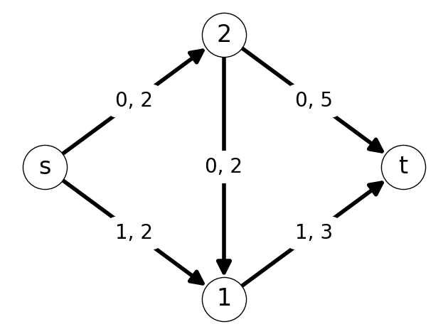
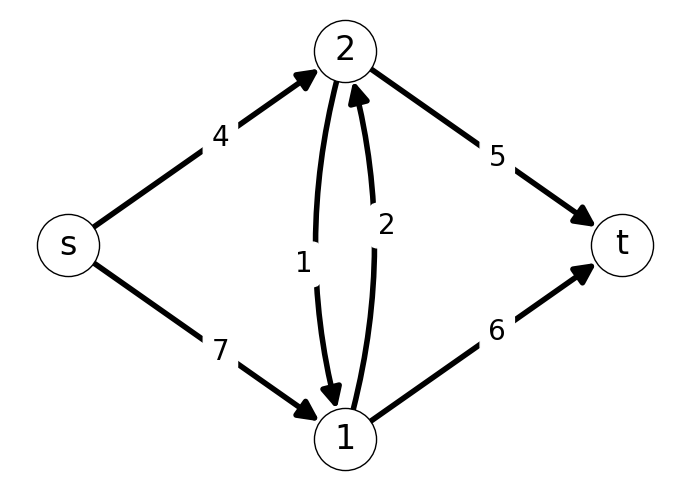
Example 7.1 Figure 7.1 gives an example of a flow \(x\) for the given graph \(G\) with capacity \(k\).
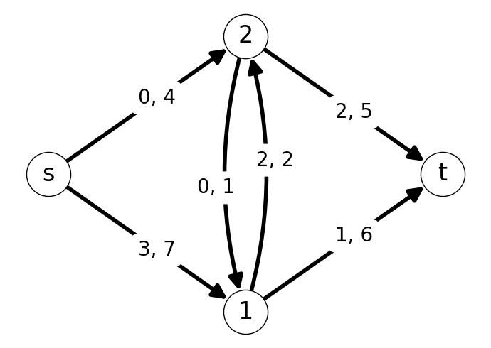
The flow can be written as \[ \begin{aligned} x_{s1} &= 3, &&& x_{s2}&=0 \\ x_{12} &= 2, &&& x_{1t} &= 1 \\ x_{21} &= 0, &&& x_{2t} &= 2. \end{aligned} \] This flow \(x\) has value \(\varphi(x) = 3.\)
7.1.5 Formulation as a Linear Program
We can write the maximum flow problem as the linear program or linear optimization problem1: \[ \begin{array}{ll} \max & \varphi \\ \text{s.t.} & \displaystyle \sum_{(h,j) \in \delta^+(h)} x_{hj} - \sum_{(i,h) \in \delta^-(h)} x_{ih}= \begin{cases} + \varphi, & \text{if } h =s, \\ - \varphi, & \text{if } h = t,\\ 0, &\text{otherwise}, \end{cases} \\ & 0 \le x_{ij} \le k_{ij} \text{ for all } (i,j) \in A, \\ & \varphi \ge 0. \end{array} \]
7.2 Cuts and Flow
7.2.1 \(st\)-cuts
Given a subset of nodes \(S \subseteq V\) with \(s \in S\) and \(t \in V \setminus S\).
Definition 7.2 An st-cut is the set of arcs that enter or leave \(S\): \[ \delta(S) = \delta^+(S) \cup \delta^{-}(S). \]
Definition 7.3 The (forward) capacity of the \(st\)-cut is \[ k(\delta(S)) = \sum_{(i,j) \in \delta^+(S)} k_{ij}. \]
7.2.2 Net Flow across a Cut
Definition 7.4 The net flow across \(\delta (S)\) is \[ \varphi(\delta(S)) := \sum_{(i,j)\in \delta^+(S)} x_{ij} - \sum_{(i,j) \in \delta^{-}(S)} x_{ij}. \]
7.2.3 Example
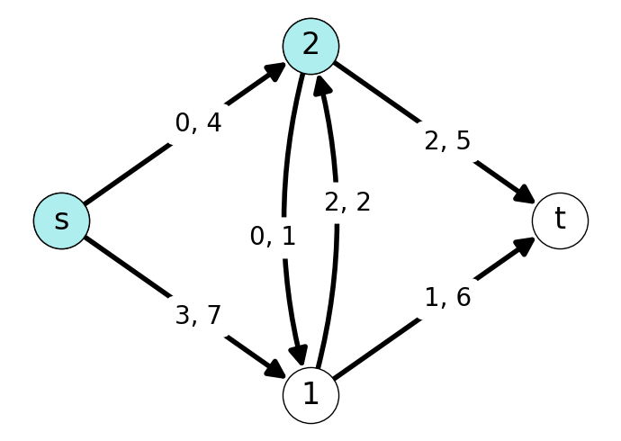
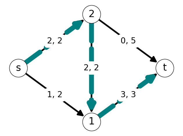
Example 7.2 Consider the graph given in Figure 7.2.
The forward and backward cuts induced by \(S\) are given in Figure 7.3.
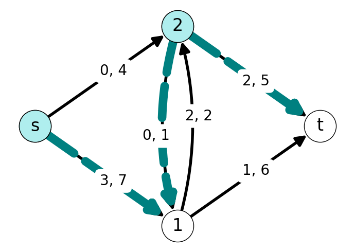
The \(st\)-cut induced by \(S\) is \[ \delta(S) = \delta^{+}(S) \cup \delta^{-}(S) = \{(s,1), (2,1), (2,t), (1,2)\}. \] The forward capacity of this cut is \[ k(\delta(S)) = 7 + 1 + 5 = 13. \] The value of this cut is \[ \varphi(\delta(S)) = 3 + 0 + 2 - 2 = 3. \]
7.2.4 Conservation of Flow Across Cuts
Lemma 7.1 Given a flow \(x\) with net value \(\varphi\), we have \[ \varphi(\delta(S)) = \varphi \] for every \(S \subseteq V\) with \(s \in S\), \(t \in V \setminus S\).
Consider the balance constraint \[ \sum_{(h,j) \in \delta^+(h)} x_{hj} - \sum_{(i,h) \in \delta^-(h)} x_{ih}= \begin{cases} + \varphi, & \text{if } h =s, \\ - \varphi, & \text{if } h = t,\\ 0, &\text{otherwise}. \end{cases} \] Let’s take the sum of both sides over all \(h \in S\); note that \(s \in S\) and \(t \notin S\). First, the sum of the right-hand side over \(h \in S\) is equal to \(\varphi\).
Next, each arc \((i,j)\) with \(i,j \in S\) appears twice in the sum on the left-hand side:
- When \(h =i\), we add \(+x_{ij}\) to the total.
- When \(h = j\), we add \(-x_{ij}\) to the total.
These two values cancel when we take the sum over all \(h\). On the other hand, if \(i\in S\) and \(j \in V \setminus S\), then \((i,j) \in \delta^{+}(S)\) and appears once in the sum of the left-hand side (when \(h=i\)). Finally, if \(i \in V \setminus S\), \(j \in S\) then \((i,j) \in \delta^-(S)\) and this edge contributes \(-x_{ij}\) to the sum in the left-hand side. Putting everything together, we have \[ \sum_{(i,j)\in\delta^+(S)} x_{ij} - \sum_{(i,j)\in\delta^-(S)} x_{ij} = \varphi. \] This completes the proof.
7.3 Duality
7.3.1 Weak Duality
The following theorem gives an upper bound on the value of any flow in terms of the capacity of an arbitrary cut. Specifically, the value of any flow is at most the capacity of any \(st\)-cut.
Theorem 7.1 For each \(S \subseteq V\) with \(s \in S\) and \(t \in V\setminus S\), we have \[ \varphi(x) \le k(\delta(S)) \] for any flow \(x\).
Let \(x\) be a feasible flow and consider \(st\)-cut \(S\). Then \[ \sum_{(i,j)\in\delta^+(S)} x_{ij} \le \sum_{(i,j)\in\delta^+(S)} k_{ij} \] since \(x_{ij}\) k_{ij}$ for any arc \((i,j)\). On the other hand, \[ - \sum_{(i,j)\in\delta^-(S)} x_{ij} le 0, \] since \(x_{ij} \ge 0\) for any arc \((i,j)\). Applying conservation of flow, Lemma 7.1, we have \[ \varphi = \sum_{(i,j)\in\delta^+(S)} x_{ij} - \sum_{(i,j)\in\delta^-(S)} x_{ij} \le \sum_{(i,j)\in\delta^+(S)} k_{ij} = k(\delta(S)). \]
7.3.2 The Minimum Cut Problem
Theorem 7.1 holds for every \(st\)-cut. In particular, it is true for the cut with minimum capacity. Thus, for any feasible flow \(x\), we have \[ \varphi(x) \le \Big\{ k(\delta(S)): \delta(S) \text{if a $st$-cut}\Big\}. \]
::: {#def-7-min-cut-problem}
7.3.2.1 Minimum Cut Problem
Given a directed graph \(G = (V, A)\) with arc capacity function \(k: A \mapsto \mathbf{R}_+\) and two nodes \(s,t \in V\).
Example 7.3 Consider the graph given in Figure 7.1. Find an \(st\)-cut of minimum capacity.
7.3.3 Strong Duality: Max-Flow Min-Cut Theorem
The relationship \[ \begin{aligned} & \varphi \le k(\delta(S)) \text{ for all $st$-cuts} \\ & \Leftrightarrow \;\;\; \varphi \le \min_S \Big\{k(\delta(S)): \delta(S) \text{ is a $st$-cut}\Big\} \end{aligned} \] holds for all net flow values \(\varphi\).
This implies that for any flow value \(\varphi\) we have \[ \varphi \le \max \Big\{\varphi(x): x \text{ is a flow}\Big\} \le \Big\{ k(\delta(S)): \delta(S) \text{if a $st$-cut}\Big\}. \]
The maximum flow value and minimum cut capacity are actually guaranteed to agree for every flow network. We have the following two results.
Lemma 7.2 Consider flow \(x\) of net value \(\varphi\) and \(st\)-cut \(\delta(S)\) of capacity \(k(\delta(S)).\)
If \(\varphi = k(\delta(S))\), then \(x\) is a maximum flow and \(\delta(S)\) is a minimum cut.
Theorem 7.2 The value of a maximum flow is always equal to the capacity of a minimum \(st\)-cut.
We’ll construct an algorithmic proof: we’ll present an algorithm that reveals and constructs the flow and \(st\)-cut while solving the problem.
7.4 The Ford-Fulkerson Algorithm – Idea
7.4.1 Improving Flows along Forward and Backward Arcs
Idea: Starting from given flow \(x\), we will try to find an \(st\)-path along which \(\varphi\) can be increased.
We can increase flow using
the original arcs in the graph (forward arcs), and
arcs whose directions have been flipped (backward arcs).
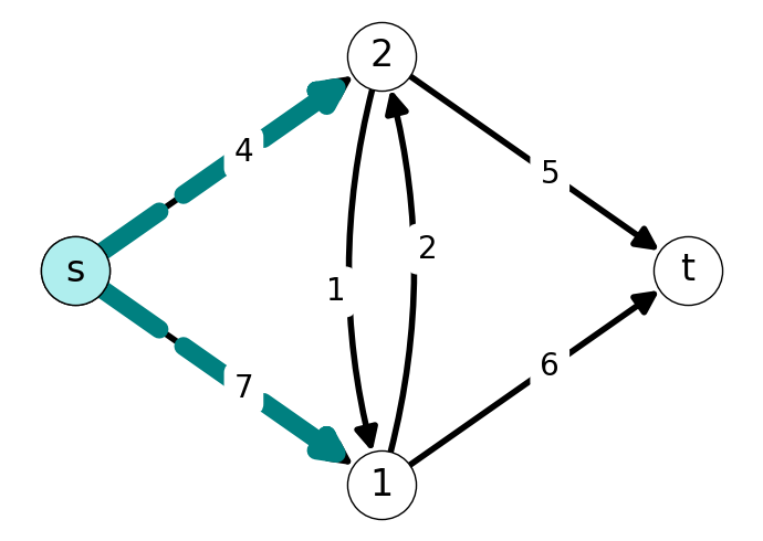
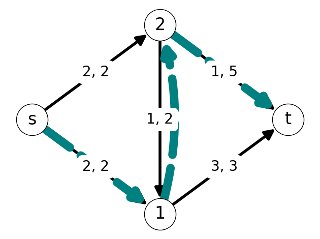
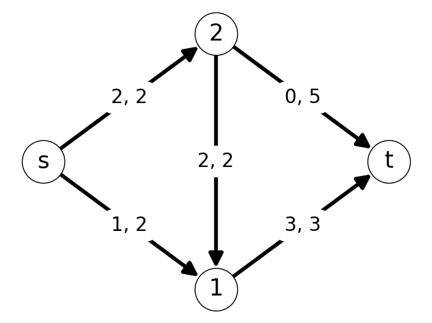
Example 7.4 Consider the graph given in Figure 7.5 (a) with flow \(x\) indicated.
We can increase the total flow by increasing by two units of flow along the forward arcs comprising the path \((s2, 21, 1t)\). This gives a new flow with value \(\varphi=3\).
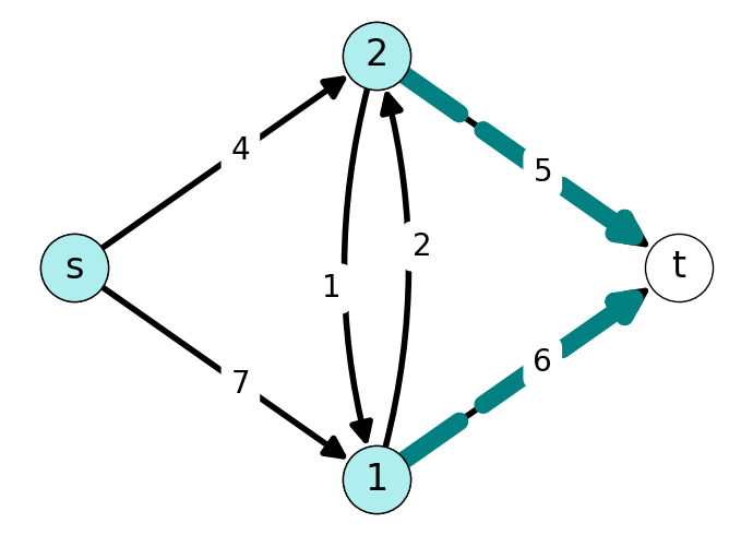
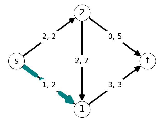
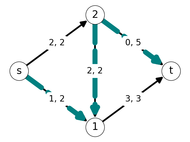
Subsequently, we can move an additional \(1\) unit of flow by redirecting \(1\) unit of flow along arc \(21\) to flow along \(2t\) and pushing an additional unit of flow along \(s1\); see Figure 7.5 (b). This is equivalent to pushing \(1\) unit of flow along the path \((s,1,2,t)\), where \(s1, 2t\) are forward arcs and \(12\) is a backward arc; see Figure 7.5 (c).
7.4.2 Saturated and Empty Arcs
Definition 7.5 An arc \((i,j)\) is saturated if \(x_{ij} = k_{ij}\).
Definition 7.6 An arc \((i,j)\) is empty if \(x_{ij} = 0\).
Observation: Our algorithm for finding the maximum flow and minimum capacity cut hinges on the following:
If \((i,j)\) is not saturated \((x_{ij} < k_{ij})\) then \(x_{ij}\) can be increased.
If \((i,j)\) is not empty \((x_{ij} > 0)\) then \(x_{ij}\) can be decreased.
Example 7.5 Consider the graph \(G\) with flow \(x\) given in @#fig-7-saturated-ex-G.
- Arcs \(s2\), \(21\), and \(1t\) are saturated;
- Arc \(2t\) is empty;
- Arc \(s1\) is not empty or saturated.

7.4.3 Augmenting Paths
Definition 7.7 (Augmenting Paths) We call a \(st\)-path using a combination of forward and backward arcs an augmenting path if:
All forward arcs are not saturated \((x_{ij} < k_{ij})\); and
All backward arcs are not empty \((x_{ij} > 0)\).
We can improve net flow value by increasing flow on forward arcs and decreasing flow on backward arcs.
Example 7.6 The graph \(G\) and flow \(x\) indicated in Figure 7.7 has augmenting path \(P=(s,1,2,t)\).
7.4.4 The Auxiliary Network
At each step of our algorithm, we will try to find an augmenting path. We will construct an additional flow network to facilitate finding such an augmenting path.
We can construct an auxiliary network \(G' = (V, A')\) with auxiliary capacity function \(k': A \mapsto \mathbf{R}_+\) that accounts for all possible flow variations with respect to current flow \(x\).
For all \((i,j) \in A\):
If \(x_{ij} < k_{ij}\) (not saturated), we add forward arc \((i,j)\) to \(A'\) with \(k'_{ij} = k_{ij} - x_{ij}\).
- This arc models the possibility of increasing the flow on \((i,j)\).
If \(x_{ij} > 0\) (not empty), we add backward arc \((j,i)\) to \(A'\) with \(k'_{ji} = x_{ij}\).
- This models the possibility of decreasing the flow on \((i,j)\).
If \(0 < x_{ij}< k_{ij}\) we add both a forward arc \((i,j)\) and a backward arc \((j,i)\) to \(A'\).
7.4.5 The Augmentation Step
Start with flow \(x\) and corresponding auxiliary network \(G'\) with auxiliary capacities \(k'\).
- Identify \(st\)-path \(P\) in \(G'\).
- Let \(\displaystyle\Delta = \min_{(i,j)\in P} k'_{ij}\).
- Add \(\Delta\) to all forward arcs.
- Subtract \(\Delta\) from all backward arcs.
7.5 Example
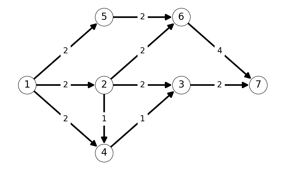
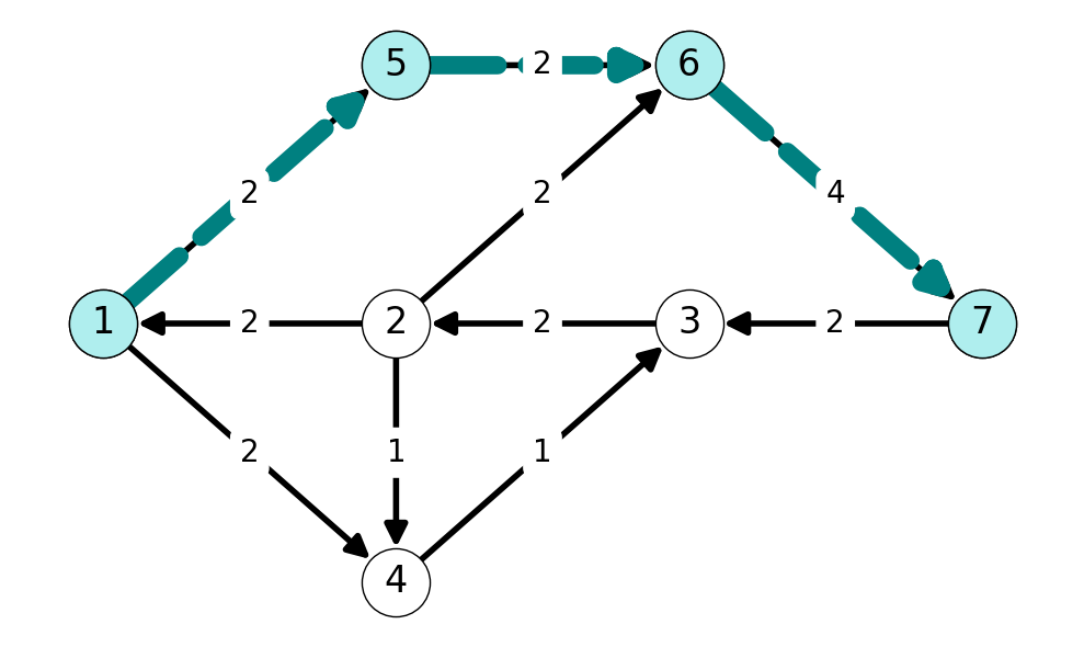
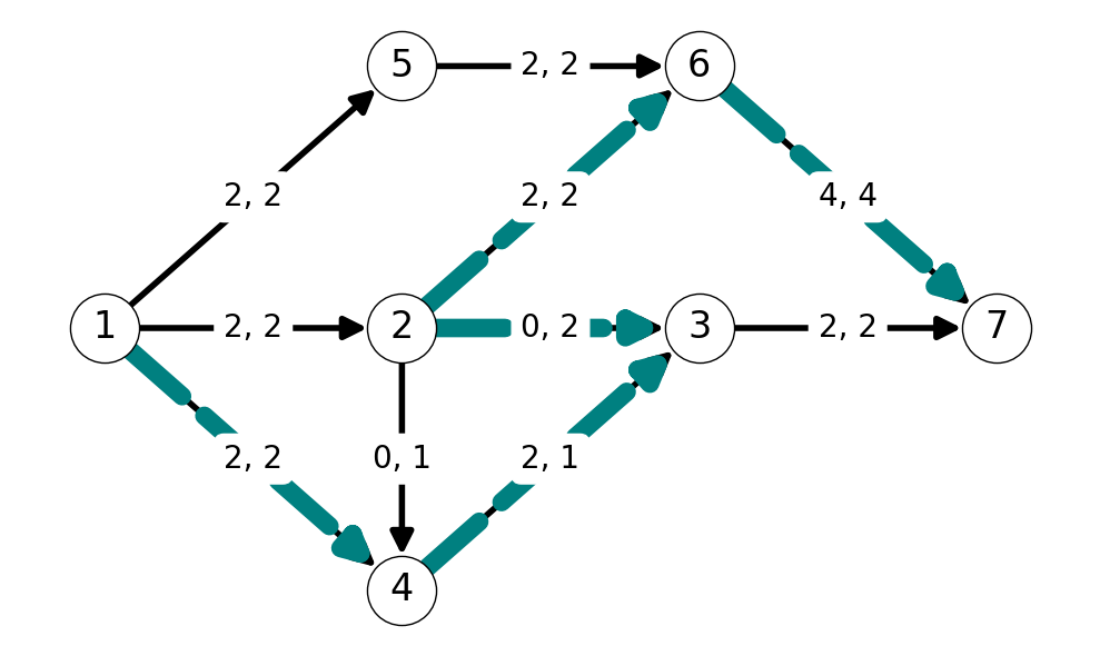
Example 7.7 Let’s find the maximum flow for \(s = 1\) and \(t=7\) for the graph Figure 7.12 (a).
We start from \(x = 0\) with net flow \(\varphi = 0\). The initial auxiliary graph \(G'\) is equal to \(G\).
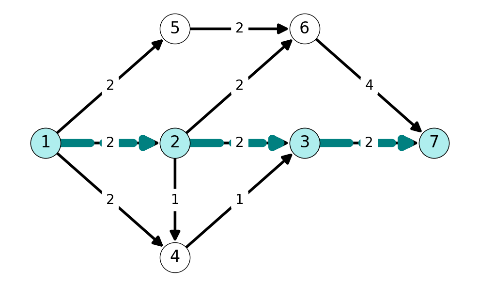
Step 1
We have several augmenting paths to choose from. Consider \(P = (1,2,3,7)\) in \(G'\). The minimum edge capacity in \(G'\) along this augmenting path is \(\Delta = 2\). All arcs in this path are forward arcs, so we add \(\Delta\) to \(x_{ij}\) for arcs \(12, 23, 37\), and leave all flow on other edges equal to \(0\).
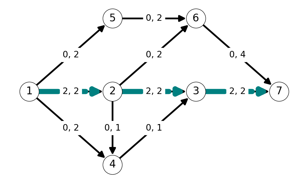
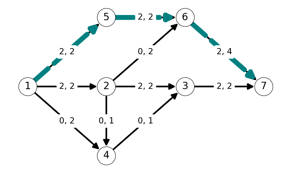
Step 2
Arcs \(12\), \(23\), and \(37\) are now saturated. We can update the auxiliary graph by reversing each of these edges and setting the capacity equal to the flow value across each arc. This reveals the augmenting path \(P = (1,5,6,7)\) (among several possible augmenting paths). This path has minimum capacity arc with capacity \(\Delta = 2\) and every arc is a forward arc on this path. Thus, we can increase flow across each of these arcs by \(\Delta=2\).
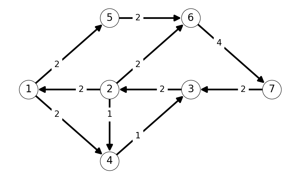
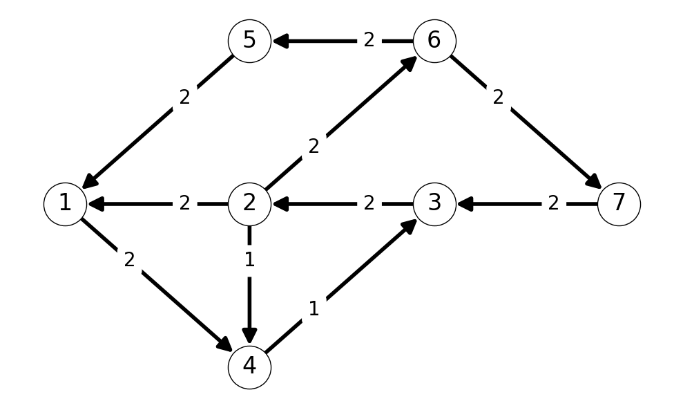
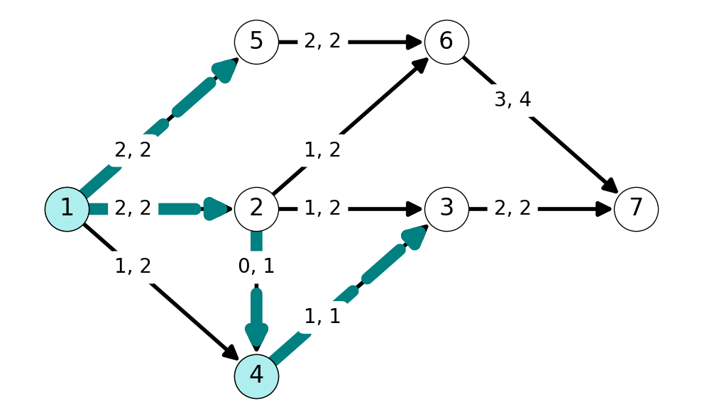
Step 3
Next, we have augmenting path \(P=(1,4,3,2,6,7)\). Note that this path uses the nonempty backward arc \(32\). The minimum capacity arc in the auxiliary graph along this path is \(43\), with capacity \(k'_{43} = 1 = \Delta\). We can update our flow by increasing the flow by \(\Delta=1\) along all forward arcs in this path and decreasing flow across backward arcs by \(\Delta=1\)
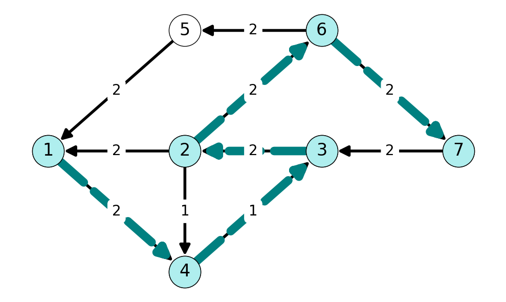
Step 4 and Termination
After updating the flow and auxiliary graph \(G'\), we can note that \(t\) is not reachable from \(s\) in \(G'\). Indeed, the reachable set from \(s\) in \(G'\) is \(S=\{s,4\}\). Note that the cut \(\delta(S)\) defined by \(S\) has capacity \(k=(\delta(S)) = 5\). This is equal to the total value of the flow \(x\) (\(\varphi = 5\)). This implies that \(x\) is a maximimum value flow and \(\delta(S)\) is a minimum capacity cut; we can stop applying the algorithm.
7.6 Termination and Correctness
7.6.1 Stopping Condition
Let \(S^*\) be the set of nodes reachable from \(s \in G'\) when the algorithm stops.
We can conclude that \(\delta_{G'}^+(S^*) = \emptyset\).
By the construction of \(G'\), this implies that:
Every arc \((i,j) \in \delta_{G}^+(S^*)\) is saturated!
Every arc \((i,j) \in \delta_{G}^-(S^*)\) is empty!
7.6.2 Correctness of the FF-Algorithm
When the algorithm terminates, all arcs in \(\delta_G^+(S^*)\) are saturated and all arcs in \(\delta_G^-(S^*)\) are empty: \[ \varphi =\varphi(\delta(S^*)) = \sum_{(i,j) \in \delta^+_G(S^*)} x_{ij} - \sum_{(i,j) \in \delta^-_G(S^*)} x_{ij} = k(\delta(S^*)). \] However, we know that \[ \varphi \le \text{max flow value} \le \text{min cut value} \le k(\delta(S^*)). \]
This shows that when the algorithm terminates, we have found a flow equal in value to the capacity of an \(s,t\) cut!.
This implies that:
The flow is optimal for the maximum flow problem.
The cut is optimal for the minimum cut problem
This establishes that the Ford-Fulkerson algorithm always finds an optimal solution!
This is an algorithmic proof of the max-flow min-cut theorem.
7.7 The Ford-Fulkerson Algorithm – Pseudocode
Initialize x = 0, phi = 0.

While x is not a max flow:
    Construct auxiliary graph G' = (V, A') with capacities k_{ij}'.

    Find an st-path P in G'.

    If P does not exist: % Terminate
        STOP! x is a max flow.
    Else % Update flow.
        Delta =  min {k_{ij}': (i,j) \in P }
        phi = phi + Delta.

        For (i,j) in P:
            If (i,j) is a forward arcL
                x_{ij} = x_{ij} + \Delta
            Else
                x_{ij} = x_{ij} - \Delta
7.8 Complexity of the Ford-Fulkerson Algorithm
7.8.1 A Rough Bound on Elementary Operations
We can count the number of elementary operations used by each iteration of the Ford-Fulkerson Algorithm:
Constructing the auxiliary graph \(G'\) in Line 4 costs \(O(m+n)\) elementary operations. Indeed, we need to construct a copy of \(G\), change direction of arcs (if necessary), and update capacities. This requires a finite number of operations for each arc and node.
We can find an \(st\)-path, if one exists, using a modification of the graph reachability algorithm. This requires \(O(m+n)\) elementary operations.
The remaining steps in the loop require \(O(|P|)\) elementary operations for augmenting path \(P\). Assuming that \(P\) is a simple path, we have \(|P| \le n-1\) edges.
Therefore, each iteration of the Ford-Fulkerson Algorithm requires \(O(m)\) elementary operations (assuming \(n = O(m)\)). If the algorithm uses \(q\) iterations, then the total number of operations is \[ O(qm). \]
7.9 Worst-Case Analysis of the Number of Iterations
To bound the number of operations needed by the Ford-Fulkerson Algorith, we need to determine how many iterations are needed by the Ford-Fulkerson Algorithm in worst-case?
The following lemma will help determine an upper bound on the number of iterations needed.
Lemma 7.3 If all capacities \(k_{ij}\) are integer then \(k_{ij}'\), \(\Delta\), and \(x\) are integer at each iteration.
Since \(\Delta\) is integer, we could have unit increment \(\Delta = 1\) each iteration (in worst case). More precisely, there are graphs where \[ \Delta = \min_{ij} k_{ij}' = 1 \] every iteration of the Ford-Fulkerson Algorithm. In this case, if we start with flow value \(\varphi=0\) then we need \(q = \varphi^*\) iterations, where \(\varphi^*\) is the value of the maximum flow.
On the other hand, if \(\Delta\) is integral and positive every iteration, then we increment \(\varphi\) by at least \(\Delta\) each iteration. Therefore, \(q \le \varphi^*\) if the capacities are integral.
It follows that the worst-case complexity of the Ford-Fulkerson Algorithm is \(O(\varphi^* m )\).
7.9.1 A Pathologically Bad Example
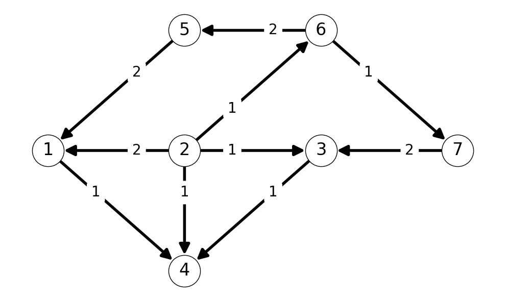
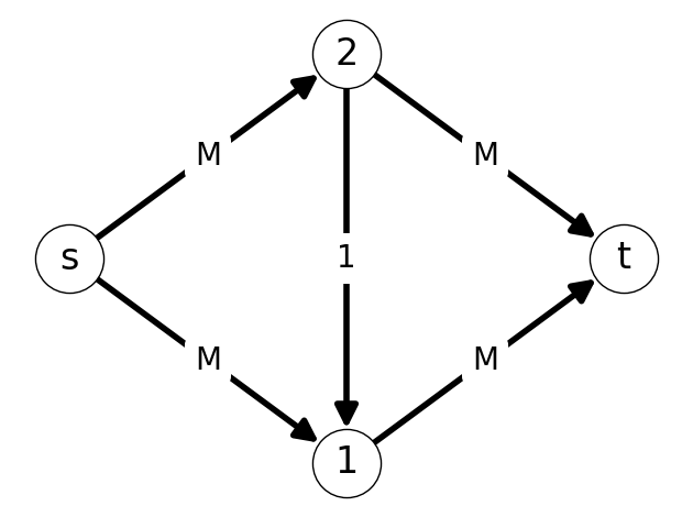
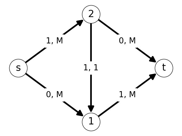
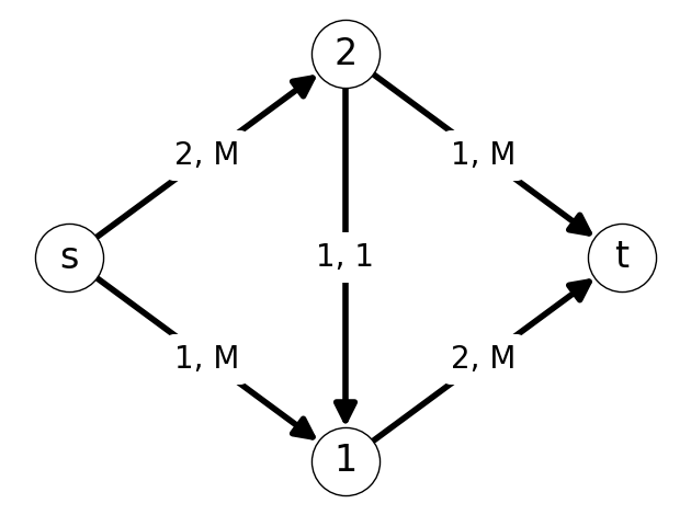
Example 7.8 Let’s apply the Ford-Fulkerson Algorithm with the graph \(G\) given in Figure 7.13 and initial flow \(x=0\).
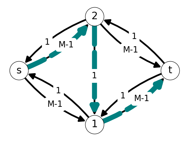
We increase flow by \(\Delta=1\) along the augmenting path \(P = (s,2,1,t)\) (Figure 7.17 (a)) This yields the new flow given in Figure 7.14 (b).
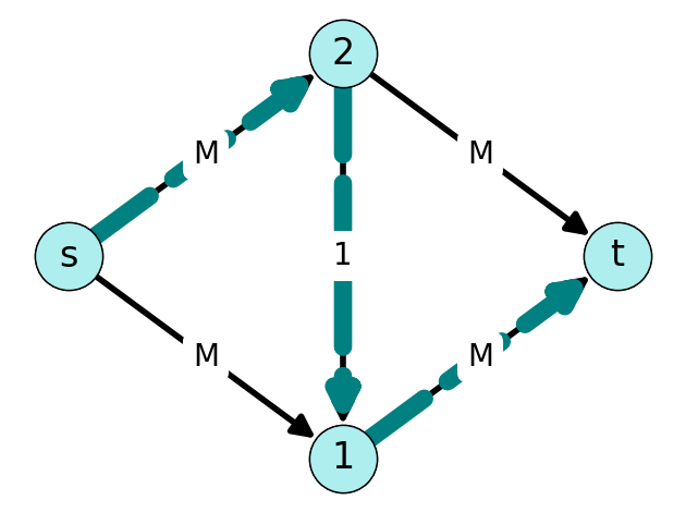
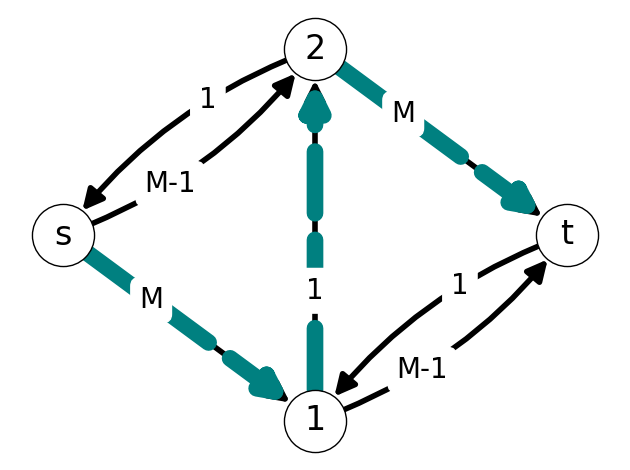
After updating the flow, we need to update the auxiliary graph. This reveals the augmenting path \(P=(s,1,2,t)\). We can increase the flow along this path by \(\Delta=1\). See Figure 7.15.
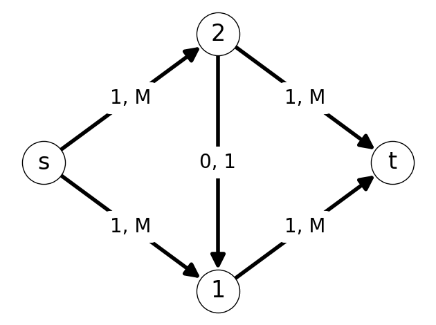
We can repeat this process. In the next step, we have augmenting path \(P=(s,2,1,t)\); this is the same augmented path used in Step 1. We can increase flow by \(\Delta=1\). In the fourth step, we increase flow by \(1\) along the augmenting path \(P=(s,1,2,t)\).
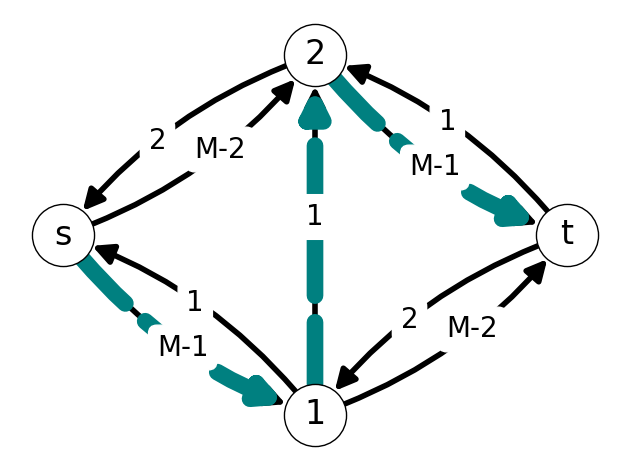
We can repeat this process a total of \(M\) times (\(2M\) iterations). This gives optimal flow given in
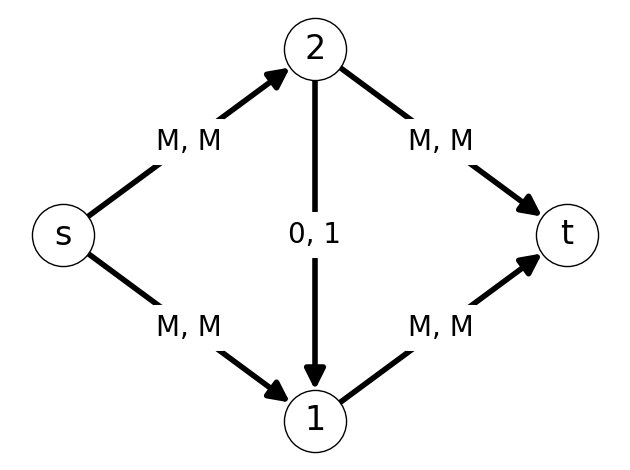
Applying the Ford-Fulkerson Algorithm with this graph requires exactly \(q = 2M = \varphi^*\) iterations.
7.9.2 Does the FF Algorithm Run in Polynomial Time?
We have deduced that the Ford-Fulkerson algorithm has complexity of \(O(\varphi^* m)\).
It is unclear whether \(O(\varphi^* m)\) a polynomial of the instance size.
Unfortunately, we can’t bound \(\varphi^*\) as a polynomial of \(n\) and/or \(m\).
Question: how should we represent the size of \(\varphi^*\)?
7.9.3 Aside: Binary Encoding
We’ll use binary encoding of numbers in our model of complexity.
Binary encoding is a positional notation system with base \(2\):
Uses two symbols: \(0\) and \(1\).
It is positional: same symbol represents different orders of magnitude based on relative position.
Digit/symbol is called a bit.
Example 7.9 Let’s convert the base-2 or binary encoding \(100110\) to base-10: \[ \begin{aligned} (100110)_{10} &= 0 \cdot 2^0 + 1 \cdot 2^1 + 0\cdot 2^3 + 0 \cdot 2^4 + 1 \cdot 2^5 \\ &= 2 + 4 + 32 = 38. \end{aligned} \]
Theorem 7.3 Given a base-10 number \(n\), we need \[ \lfloor{\log n \rfloor} + 1 = O(\log n) \] bits to encode it in base-2.
Example 7.10 For example, \[ (38)_{10} = (100110)_{2} \] requires \[ \lfloor\log_2(38)\rfloor \approx \lfloor 5.25\rfloor + 1 = 6 \] bits of storage.
7.9.4 Storage Needs of the Maximum Flow Problem
For an instance of the maximum flow problem, we need to store the graph topology, i.e., nodes and adjacencies encoded by arcs, and the capacity value per arc.
We can extend our notion of an adjacency list to keep track of indices and arc capacities. We will store the capacity of an arc using tuples in a list for each node. This is illustrated in the following example.
Example 7.11 Consider the graph given in Figure 7.19. We can encode the edges within the adjacency list. For example, nodes \(2\) and \(t\) are both adjacent \(1\), by arcs with capacities \(2\) and \(6\) respectively. We can encode this using a modified adjacency list \[ L(1) = \{(2,2), (t,6)\}. \] We can construct adjacency lists for each remaining node using an identical process: \[ \begin{aligned} L(s) &= \{(1,7), (2,4)\}, \\ L(2) &= \{(1,1), (t,5)\}, \\ L(t) &= \emptyset. \end{aligned} \]
7.9.5 Instance Size of Maximum Flow
Arc \((i,j)\) corresponds to an entry in adjacency sublist \(L(i)\).
Using a binary encoding, each entry contains:
The index \(j \in \{1,\dots, n\}\) encoded using \[ \lfloor{\log j \rfloor} + 1 = O(\log j) = O(\log n)\text{ bits,} \] since \(\log j = O(\log n)\).
The capacity \(k_{ij}\) of arc \((i,j)\) encoded using \[\lfloor{\log k_{ij} \rfloor} + 1 = O(\log k_{\max}) \text{ bits,}\] where \(k_{\max} := \max\left\{k_{ij}: (i,j) \in A \right\}\).
This totals \(O\Big(m \big(\log n + \log k_{\max} \big) \Big)\) bits.
Example 7.12 Consider the graph \(G\) given in Figure 7.13. Recall, that solving the maximum flow problem using the Ford-Fulkerson Algorithm has complexity \(O(\varphi^*)\). We’d like to know how this complexity \(O(\varphi^*)\) compares to instance size \(O(m(\log n + \log k_{\max}))\).
Recall that \(\varphi^* = 2M\) for this example. Moreover, \(k_{\max} = M\). Unfortunately, the instance size depends logarithmically on \(k_{\max}\), not linearly. Indeed, \[ k_{\max} = 2^{\log_2 (k_{\max})}. \] This implies that \[ O(\varphi^* m = O(k_{\max} m) = O\left( 2^{\log k_{\max}}\cdot m \right), \] which grows exponentially in \(\log (k_{\max})\).
On the other hand, the instance size \(O(m(\log n + \log k_{\max}))\) grows linearly in \(\log (k_{\max})\).
Therefore, \(O(\varphi^* m)\) is not a polynomial function of the instance size. Therefore, the Ford-Fulkerson Algorithm is not polynomial in complexity.
7.9.6 The General Case
This example establishes that the Ford-Fulkerson Algorithm is not polynomial.
We can generalize the complexity of the FF algorithm without relying on \(\varphi^*\). To avoid using \(\varphi^*\), which is usually not known, we can substitute an upper bound on \(\varphi^*\).
Example 7.13 As a simple example, consider a graph with maximum capacity \(k_{\max}\) and \(m\) arcs. Then \[ \varphi^* \le m k_{\max} \] since each arc cannot carry more flow than \(k_{\max}\) and there are \(m\) arcs. This gives the upper bound on complexity \[ O(\varphi^* m) \le O\left( (k_{\max} m) \cdot m \right) = O\left(k_{\max} m^2 \right). \] Unfortunately, this upper bound is tight: there are graphs \(G\) for which the Ford-Fulkerson Algorithm uses \(\varphi^* = k_{\max} m\) iterations.
7.9.7 Pseudopolynomiality
The complexity \(O(k_{\max} m^2)\) is not polynomial if we assume a binary encoding because \(k_{\max} = O(2^{\log k_{\max}})\).
However, the instance size is polynomial with respect to instance size if we use a unary encoding (encode integers using only \(1\)s):
- For example, \(7\) is encoded in unary as \(1111111\).
Using a unary encoding, we need:
\(O(mn)\) symbols to store the graph topology, and
\(O(mk_{\max})\) symbols to store the arc capacities.
We call such an algorithm pseudopolynomial.
7.9.8 Polynomial-Time Algorithms for Maximum Flow
Strongly polynomial algorithms do exist for the maximum flow problem. The Edmonds/Karp algorithm23 is the most widely used example, but is beyond the scope of this course.