9 Complexity of Problems

9.1 Complexity Classes

9.1.1 Problem Complexity

Recall the Cobham-Edmonds thesis¹: \(P\) is tractable or well-solved if

There is an algorithm \(A\) which solves it.
\(A\) has computational complexity which is a polynomial function of the instance size of \(P\).

We have seen several problems which are tractable:

minimum spanning tree
shortest path
max flow / min cut problem
matching (unweighted, weighted, and assignment).

Indeed, we have developed and analysed polynomial time algorithms for each of these problems earlier in the module.

A foundational question in complexity theory is whether there are inherently difficult problems which cannot be solved in polynomial time?

There are many problems that nobody knows how to solve in polynomial time.
This doesn’t mean that it is impossible to solve them in polynomial time.
It just means we haven’t found a polynomial time algorithm yet.

9.1.2 The PRIME Problem

PRIME: given an integer \(k\), is \(k\) prime?

It was thought that PRIME did not have a polynomial time algorithm for a long time. However, Agrawak, Kayal, and Saxena² found one in 2002 that requires \(O \Big( (\log k)^{12} \big( \log (\log k)^{12}\big)^c\Big)\) elementary operations, for some \(c \ge 1\).

9.1.3 Goals of Complexity Theory

We want to build a theory that allows us to conclude that a problem does not have a polynomial time algorithm.

The best we can do today is develop theory that let’s us conclude that a problem is very unlikely to have a polynomial time algorithm.

9.1.3.1 The Traveling Salesperson Problem (TSP)

We will repeatedly reference the traveling salesperson problem as an illustrative example.

Definition 9.1 A Hamiltonian circuit or cycle or tour of direted graph \(G = (V,A)\) is a cycle that visits each node exactly once

Definition 9.2 Traveling Salesperson Problem (TSP):³

Given graph \(G\) with arc costs \(c_{ij} \in \mathbf{Z}_+\).
Find a Hamiltonian cycle of \(G\) with minimum cost.

The TSP has many applications, especially within logistics/transportation, circuit design, and scheduling.

9.1.4 Types of Problems

Given problem instance \(I\) defined by set of feasible solutions \(F\) and cost function \(c: F \mapsto \mathbf{R}\).

Definition 9.3 (Decision Problem)

Given \(L \in \mathbf{R}\), is there \(X \in F\) such that \(c(X) \le L?\)
Algorithm \(A\) takes input \(I, L\) and returns YES or NO.
Search version: \(A\) returns \(X \in F\) with \(c(X) \le L\) if one exists.

Definition 9.4 (Optimization Problems in Search Version)

Algorithm \(A\) finds \(X \in F\) minimizing \(c(X)\).

Example 9.1 (Versions of TSP) We can formally define two versions of the TSP:

TSP as an Optimization Problem:
- Given directed graph \(G = (V,A)\) with costs \(c_{ij} \in \mathbf{Z}_+\) for each arc \((i,j) \in A\):
- Find a Hamiltonian cycle with minimum total cost.
TSP as a Decision Problem
- Given directed graph \(G\), arc costs \(c_{ij}\), and integer \(L\):
- Does \(G\) contain a Hamiltonian cycle of total cost at most \(L\)?

9.1.5 Comparison of Complexity of Decision and Optimization Problems

This prompts a reasonable question:

Which is inherently more difficult?
Optimization or decision problems?

The following theorem answers this fundamental question.

Theorem 9.1 Any algorithm \(A\) for an optimization problem \(P\) solves the decision version \(P_d\).

Theorem 9.1 has a natural corollary, which establishes that tractable optimization problems correspond to tractable decision problems.

Corollary 9.1 If the optimization problem \(P\) is polynomial time solvable, then the decision problem \(P_d\) is also polynomial time solvable.

Proof. We have the following algorithm for solving the decision problem \(P_d\) given an algorithm \(A\) for solving optimization problem \(P\):

Solve \(P\) using \(A\). Let \(X^*\) be the minimizer of \(P\) with minimum value \(c(X^*)\).
Compare the optimal value to \(L\):
- Return YES if \(c(X^*) \le L\);
- Otherwise, return NO.

If \(A\) is polynomial time then this algorithm is also polynomial time.

We aim to categorize decision problems based on their inherent difficulty.

We will start by comparing two complexity classes, \(\mathbf{P}\) and \(\mathbf{NP}\).

9.1.6 The Class \(\mathbf{P}\)

Definition 9.5 We denote by \(\mathbf{P}\) the class of all decision problems which can be solved in polynomial time for every instance \(I\)⁴.

We have seen several examples of problems belonging to \(\mathbf{P}\). Indeed, the decision versions of the minimum spanning tree, shortest path, max flow, matching, and assignment problems are all in \(\mathbf{P}\).

9.1.7 The Class \(\mathbf{NP}\)

Definition 9.6 We say a problem \(\mathbf{NP}\) belongs to the complexity class P or nondeterministic polynomial⁵ if:

Every instance \(I\) of \(P \in \mathbf{NP}\) with answer YES (called a YES-instance), has a certificate which verifies that the instance has answer YES in polynomial time.

We are not interested in how to build the certificate; just whether we can verify in polynomial time.

Example 9.2 (Complexity Class of TSP) The Traveling Salesperson Problem is in \(\mathbf{NP}\).

To see that TSP is in \(\mathbf{NP}\), we need to identify a certificate for an arbitrary YES-instance.

Consider the following proposed certificate for instance of TSP with \(G = (V,A)\) and threshold \(L\):

Let \(S = (v_1, v_2, \dots, v_n)\) be a sequence of nodes such that
1. \(S\) contains all nodes of \(G\) exactly once.
2. Pairs of consecutive nodes share an arc: \((v_i, v_{i+1}) \in A\). Moreover, \((v_n, v_1) \in A\).
3. Total cost of these arcs is \[ \sum_{i=1}^n c((v_i, v_{i+1})) \le L; \] here, we use \(v_{n+1} = v_1\).

This is a certificate! If given \(S\), we can that check that (1), (2), and (3) are satisfied in polynomial time.

Indeed, \(S\) and \((v_n, v_1)\) define the desired Hamiltonian cycle in this case.

9.1.8 Differences between \(\mathbf{P}\) and \(\mathbf{NP}\)

The class \(\mathbf{P}\) contains polynomial time solvable problems:

\(\mathbf{P}\) contains decision problems to which a YES/NO answer can be given for any instance in polynomial time.

Other other hand, \(\mathbf{NP}\) contains polynomial time certifiable problems:

YES-instances admit a certificate which can be verified in polynomial time.

9.1.9 Turing Machines

Definition 9.7 A turing machine (TM)⁶ is a mathematical model of computer as an abstract machine that:

manipulates symbols from an infinite tape (can read and write),
according to table of rules implementing a finite-state automaton⁷.

Everything a computer can do can be modeled by a TM.

\(\mathbf{P}\) is the set of problems that can be solved in polynomial time by a TM.
\(\mathbf{NP}\) is the class of problems that can be solved (not just certified) in polynomial time by a nondeterministic TM⁸.

9.1.10 The Relationship Between \(\mathbf{P}\) and \(\mathbf{NP}\)

It is known that \(\mathbf{P}\) is a subset of \(\mathbf{NP}\). That is, every problem in \(\mathbf{P}\) also belongs to \(\mathbf{NP}\).

We have the following theorem.

Theorem 9.2 \(P \subseteq NP\)

Proof. Suppose that problem \(Q\) in \(\mathbf{P}\), i.e., \(Q \in \mathbf{P}\). This implies that there is a polynomial time algorithm \(A\) for \(Q\).

The steps of \(A\) act as a certificate:

If \(A\) solves search version of \(Q\), then the solution returned by \(A\) satisfies the conditions for YES response.
If \(A\) only returns YES or NO applying \(A\) and obtaining response YES is the certificate.

9.1.10.1 Does \(\mathbf{P} = \mathbf{NP}\) or \(\mathbf{P} \neq \mathbf{NP}?\)

Conjecture 9.1 It is widely conjectured that there is at least one problem in \(\mathbf{NP}\) but not in \(\mathbf{P}\), i.e., \(\mathbf{P} \neq \mathbf{NP}\).

Falsifying Conjecture 9.1 would prove that \(\mathbf{P} = \mathbf{NP}\).
Determinining if \(\mathbf{P} = \mathbf{NP}\) or \(\mathbf{P} = \mathbf{NP}\) is one of the seven Millenium Prize Problems⁹.

9.2 Reductions

9.2.1 Turing and Cook Reductions

Suppose we are given two decision problems \(P\) and \(Q\).

Definition 9.8 (Turing Reduction) There is a Turing reduction from \(P\) to \(Q\), denoted \(P \le_T Q\) if \(P\) can be solved by an algorithm that calls algorithm \(A_Q\) for solving \(Q\) as a subroutine.

Example 9.3 (Maximum Matching and Network Flow) Let \(P\) and \(Q\) be the decision versions of maximum matching and network flow respectively:

\(P\): does graph \(G\) have a matching of cardinality \(\ge k\)?
\(Q\): does flow network \(G\) have a flow with value \(\ge k\)?

We saw in Problem Set 7 that every instance of the maximum matching problem translates to a special case of the maximum flow problem.

Thus, we can solve instances of \(P\) using algorithms for max flow and/or min cut. It follows that \[ \quad P \leq_T Q. \]

Definition 9.9 (Cook Reduction) There is a polynomial or Cook reduction, denoted \(P \le_T^P Q\), from \(P\) to \(Q\) if

\(P\) can be solved by an algorithm \(A_P\) that calls algorithm \(A_Q\) for solving \(Q\) as a subroutine; and
\(A_P\) would run in polynomial time if we assume that \(A_Q\) has complexity \(O(1)\).

This requires that the number of calls to \(A_Q\) is polynomial, and all other operations in \(A_P\) run in polynomial time.
Cook reductions are a special case of Turing reductions.

If \(P \le_T^P Q\) and \(A_Q\) has complexity \(O(1)\) then \(P\) is solvable in polynomial time using the polynomial reduction.

Theorem 9.3 Suppose that \(P \le_T^P Q\). If \(Q \in \mathbf{P}\) then \(P \in \mathbf{P}\).

9.2.2 Mapping Reductions and Polynomial Transformations

Definition 9.10 There is a mapping reduction from \(P\) to \(Q\) (\(P\le_m Q\)) if there is a Turing reduction from \(P\) to \(Q\) in which \(A_Q\) is called only once.

In a mapping reduction, each instance of \(P\) is transformed into an instance of \(Q\) and solved with \(A_Q\).

Definition 9.11 (Karp Reductions) There is a polynomial mapping reduction or Karp reduction from \(P\) to \(Q\) (\(P \le_m^P Q\)) if there is a polynomial reduction from \(P\) to \(Q\) in which \(A_Q\) is called only once.

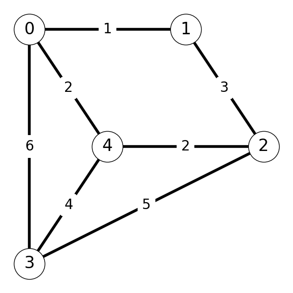
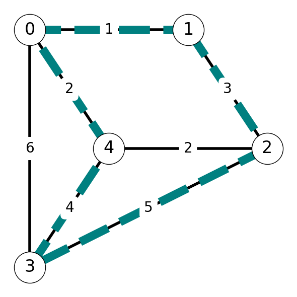
Example 9.4 (Reductions for TSP) Consider the following versions of the TSP:

UTSP-d: Given an undirected graph with edge cost function \(c\) and integer \(L\), is there a Hamiltonian cycle with cost \(\le L\)?
TSP-d: Given a directed graph with arc cost function \(c\) and integer \(L\), is there a Hamiltonian cycle with cost \(\le L\)?

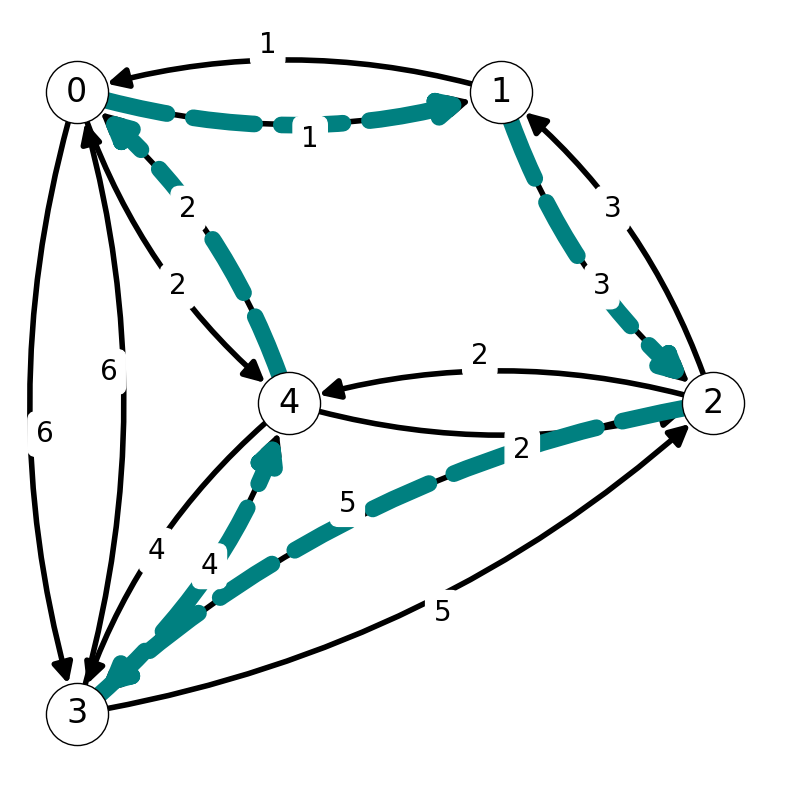
Consider the instances of UTSP-d given in Figure 9.1. We can replace this instance of UTSP-d with an instance of TSP-d by creating two directed arcs \((i,j)\) and \((j,i)\) for each edge \(ij\) in \(G\). Both the undirected and directed graphs have Hamiltonian cycle \(C = (0,1,2,3,4)\) with cost \(L = 15\).

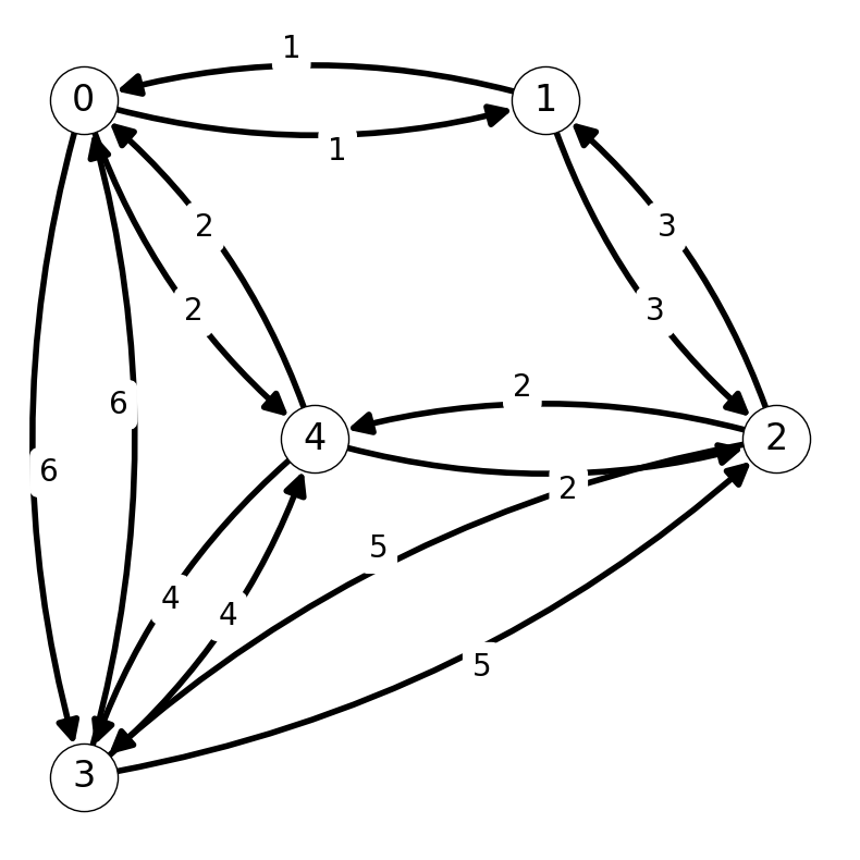
Let’s generalize this phenomena. Let \([G=(V,E), L]\) be an instance of UTSP-d.

We transform it into an instance of TSP-d \([G'=(V',E'), L']\) as follows:

\(V'=V\);
let \(E'\) beset of arcs containing a pair of anti-parallel arcs for each edge in \(E\) with same cost; i.e., add \((i,j)\) and \((j,i)\) to \(E'\) for each \(ij\) in \(E\) with cost \[ c'_{ij} = c_{ij} = c'_{ji}. \]

Under this construction, \([G=(V,E), L]\) has answer YES if and only if \([G'=(V',E'), L']\) has answer YES. Indeed:

If \(G\) is a YES instance then follow its tour, either clockwise or anticlockwise, to get a directed tour in \(G'\). This implies that \(G'\) is a YES instance too!
If \(G'\) is a YES instance then selecting arcs from its Hamiltonian cycle as edges in \(G\) gives a Hamiltonian cycle in \(G\). Therefore, \(G\) is a YES instance!

9.3 The NP-complete class

Definition 9.12 A decision problem \(P\) is \(\mathbf{NP}\)-complete¹⁰ if

\(P \in \mathbf{NP}\).
Every other problem in \(\mathbf{NP}\) reduces polynomially to it: \[ \text{For all } Q \in \mathbf{NP}, \;\; Q \le_T^P P. \]

Theorem 9.4 The existence of a polynomial time algorithm for any NP-complete problem would imply that \[ {\mathbf{P} = \mathbf{NP}} \]

Proof. Every problem \(Q \in \text{NP}\) reduces in polynomial time to \(R\) if \(R\) is \(\mathbf{NP}\)-complete.

If we could solve \(R\) using a polynomial-time algorithm, we could solve every \(Q \in \text{NP}\) in polynomial time, which implies that \(\mathbf{P} = \mathbf{NP}.\)

9.3.1 Consequences

We have established that problems in \(\mathbf{NP}\)-complete are more general than any problem in \(\mathbf{NP}\):

Here, generality of a problem \(Q\) follows the definition of polynomial reduction.
That is, as a measure of how many problems we could solve in polytime if we could solve \(Q\) in \(O(1)\).
If \(Q\) is \(\mathbf{NP}\)-complete this generality is maximized since all of \(\mathbf{NP}\) can be solve in polytime if \(Q\) can be solved in \(O(1)\).

9.3.2 Notions of Hardness

Suppose that we are trying to determine how hard it is to solve problem \(Q\).

Suppose that we try to construct a polynomial time algorithm but fail to find one.
Then try to show \(Q\) is \(\mathbf{NP}\)-complete and succeed.
This doesn’t prove that \(Q\) is not solvable in polynomial time.

If we could solve \(Q\) in polynomial time, then \(\mathbf{P = NP}\) and all problems in \(\mathbf{NP}\) would be polytime solvable.

If \(Q \in\)\(\mathbf{NP}\)-complete, then \(Q\) must be as hard as all other problems nobody knows how to solve in polytime.

9.4 Constructing Turing Reductions

We can use polynomial reductions to prove that a problem is \(\mathbf{NP}\)-complete.

Theorem 9.5 Given problem \(P \in \mathbf{NP}\).

Suppose that there is \(\mathbf{NP}\)-complete problem \(Q\) which reduces to \(P\).
Then \(P\) is also \(\mathbf{NP}\)-complete.

Issue: To show that \(P\) is \(\mathbf{NP}\)-complete, we need to know and use at least one other \(\mathbf{NP}\)-complete problem!

Proof. Suppose that \(Q\) is \(\mathbf{NP}\)-complete:

\(Q \in \mathbf{NP}\);
\(R \le_T^P Q\) for all \(R \in \mathbf{NP}\).

Now suppose that \(Q\) reduces to \(P \in \mathbf{NP}\): \(Q \le_T^P P\). Then, we have \[ R \le_T^P Q \le_T^P P \] for every problem \(R \in \mathbf{NP}\). Therefore, \(R \le_T^P P\) and, hence, \(P\) is \(\mathbf{NP}\)-complete.

9.4.1 The Satisfiability (SAT) Problem

Given \(n\) Boolean variables \(Y_1, Y_2, \dots, Y_n\) and \(m\) Boolean clauses \(C_1, \dots, C_m\).

Is there a truth assignment (TA) SATisfying all of the clauses?

We call the occurrences of variable \(Y_i\) in a clause literals.
These are either positive \((Y_i)\) or negative \((-Y_i)\).
\(\vee\) denotes or in each clause.

Theorem 9.6 (Cook 1971) SAT is \(\mathbf{NP}\)-complete.

Example 9.5 Consider an instance of SAT with variables \(Y_1, Y_2, Y_3, Y_4\) and clauses:

\(C_1: (Y_2 \vee Y_3)\)
\(C_2: (Y_1 \vee -Y_2 \vee Y_4)\)
\(C_3: (-Y_1 \vee -Y_2 \vee Y_3 \vee -Y_4)\)

We want to assign values in \(\{T, F\}\) to \(Y_1, Y_2, Y_3, Y_4\) so that \(C_1\) and \(C_2\) and \(C_3\) are all satisfied.

This is a YES-instance of SAT. Indeed:

Setting \(Y_2 = T\) satisfies \(C_1\);
Similarly, \(Y_1 = T\) ensures that \(C_2\) is satisfied;
Finally, setting \(Y_3 = T\) and/or \(Y_4 = F\) satisfies \(C_3\).

Therefore, this instance of SAT admits several solutions, including \((Y_1, Y_2, Y_3, Y_4) = (T, T, T, F)\) and \((Y_1, Y_2, Y_3, Y_4) = (T, T, T, T)\).

9.4.2 Hierarchy of Reductions

Karp 1972: 21 of most famous problems without known polytime algorithms are \(\mathbf{NP}\)-complete by reduction from SAT.

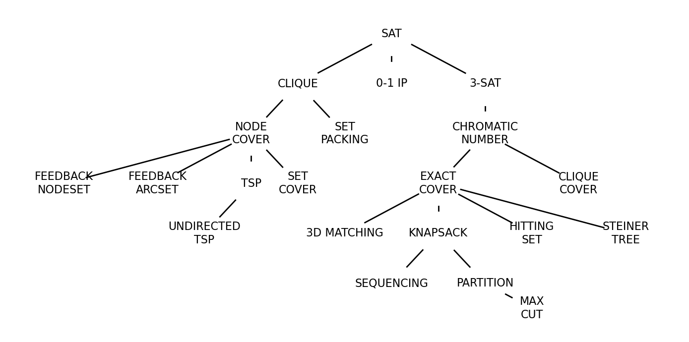
Figure 9.2: Karp’s Heirarchy of Reductions

Karp used a series of reductions from SAT to establish that each problem is \(\mathbf{NP}\)-complete.

9.4.3 The \(\mathbf{NP}\)-hard Class

Definition 9.13 We say that problem \(P\) is NP-hard if every problem in \(\mathbf{NP}\) polynomially reduces to it.

Note: \(P\) may not belong to \(\mathbf{NP}\).

9.4.4 Complexity of Optimization Problems

Theorem 9.7 If a decision problem \(P_d\) is NP-complete then its optimization counterpart \(P_o\) is NP-hard.

Proof. Recall that \(P_d\) can be solved by calling an algorithm for the optimization problem \(P_o\). Thus, \[ P_d \le_T^P P_o. \] If \(P_d\) is \(\mathbf{NP}\)-complete then every \(Q \in \mathbf{NP}\) reduces to \(P_d\): \[ Q \le_T^P P_d \le_T^P P_o. \] Therefore, every \(Q \in \mathbf{NP}\) reduces to \(P_o\). Therefore, \(P_0\) is \(\mathbf{NP}\)-hard.

Note that \(P_o\) is not in \(\mathbf{NP}\) because \(P_o\) is not a decision problem; thus, \(P_o\) is not \(\mathbf{NP}\)-complete.

9.4.5 Examples of \(\mathbf{NP}\)-hard Problems

All of the optimization counterparts of \(\mathbf{NP}\)-complete problems we have see are \(\mathbf{NP}\)-hard.

TSP (given graph \(G\) and arc costs \(c\), find Hamiltonian cycle with minimum cost) is \(\mathbf{NP}\)-hard.
Unless \(\mathbf{P}=\mathbf{NP}\), the problems in \(\mathbf{P}\) we have seen (e.g., minimum spanning tree, shortest path, matching, max flow) are not \(\mathbf{NP}\)-hard.
- If they were \(\mathbf{NP}\)-hard, every problem in \(\mathbf{NP}\) would be solvable in polynomial time by reduction to them.

9.5 Example: A Chain of Reductions

We’ll use the chain of reductions \[ \text{SAT} \Rightarrow \text{3-SAT} \Rightarrow \text{STAB-d} \Rightarrow \text{CLIQUE-d} \] to establish that each problem (except SAT) is \(\mathbf{NP}\)-complete.

(We’ll formally define these problems as we go through the chain.)

9.5.1 The 3-SAT Problem

Given:

\(n\) Boolean variables \(Y_1, \dots, Y_n\),
\(m\) Boolean clauses \(C_1, \dots, C_m\) each containing at most 3 literals.

Is there a Truth Assignment (TA) satisfying all the clauses?

The 3-SAT problem is a restriction of SAT:
- The definition of 3-SAT adds a further constraint to the definition of SAT.

Example 9.6 The following defines and instance of 3-SAT with four variables and three clauses: \[ (-Y_1\vee Y_2 \vee -Y_3) \wedge (Y_4 \vee -Y_2 \vee Y_3) \wedge (-Y_4 \vee Y_2 \vee Y_3) \] This is a YES-instance of 3-SAT: \[ (Y_1, Y_2, Y_3, Y_4) = (F, T, T/F, T) \] is a solution.

9.5.2 SAT to 3-SAT

Theorem 9.8 3-SAT is \(\mathbf{NP}\)-complete

Proof. We will prove the theorem by:

Showing that 3-SAT \(\in \mathbf{NP}\).
Showing that SAT \(\le_T^P\) 3-SAT

9.5.2.1 3-SAT \(\in \mathbf{NP}\)

Any Boolean vector in \(\{T,F\}^n\) corresponding to a TA providing answer YES is a polytime-verifiable certificate:

We can check in linear time whether each clause is satisfied.
Indeed, we compare each literal in each clause with their counterpart in the TA.
The clause is satisfied if we have:
- positive literal \(Y_i\) with \(Y_i=T\), or
- negative literal \(-Y_i\) with \(Y_i=F\).

9.5.2.2 Reduction

Suppose that we are given a SAT instance with clauses with at least \(4\) literals.

Otherwise, the SAT instance is already a 3-SAT instance.

Let’s consider the SAT clause with variables \(X_1, \dots, X_k\): \[ C_j = (x_1 \vee x_2 \vee \cdots \vee x_k). \] Each \(x_j\) is a literal (may correspond to either \(X_j\) or \(-X_j\).) We want to replace \[ C_j = (x_1 \vee x_2 \vee \cdots \vee x_k). \] by a set of 3-SAT clauses.

To do so, we introduce new variables \(Y_1, Y_2, \dots, Y_{k-3}\). We will show that \(C_j\) is equivalent to the clause \[ \tilde C = (x_1 \vee x_2 \vee Y_1) \wedge (x_3 \vee -Y_1 \vee Y_2) \wedge (x_4 \vee -Y_2 \vee Y_3) \wedge \cdots \wedge (x_{k-1} \vee x_k \vee - Y_{k-3}). \]

To see that \(C_j\) and \(\tilde C\) are equivalent, suppose that \(C_j\) is satisfied. Then \(x_j = T\) for some \(j\). We want to show that \(\tilde C\) is also satisfied. Consider \[ Y_i = \begin{cases} T, &\text{if } i =1,2,\dots, j-2, \\ F, &\text{if } i = j-1, \dots, k-3. \end{cases} \] This choice of \((x,Y)\) satisfies each of the 3-SAT subclauses in \(\tilde C\). Indeed, the clause \[ x_i \vee - Y_{i-2} \vee Y_{i-1} \] is satisfied by:

\(Y_{i-1}=T\) for \(i=1,2,\dots, j-2\);
\(-Y_{i-2}=F\) otherwise.

On the other hand, suppose that \(\tilde C\) is satisfied. We want to show that \(C_j\) is also satisfied.

We have two possible options. First, there is a \(j\) such that \(x_j = T\). Then \(C_j\) is satisfied as well.

Next, we could have \(x_j = F\) for all \(j\):

\(x_1 = x_2 = F\) implies that \(Y_1 = T\) if \(\tilde C\) is satisfied;
\(x_3 = -Y_1 = F\) implies that \(Y_2 = T\);
\(x_4 = -Y_2 = F\) implies that \(Y_3 = T\); and so on.

Iterating shows that \(Y_j = T\) for all \(j = 1,2,\dots, k-3\). However, the final 3-SAT subclause \[ -Y_{k-3} \vee x_{k-1} \vee x_k \] is not satisfied since \[ -Y_{k-3} = x_{k-1} = x_k = F. \] This implies that we must have at least one \(x_j = T\) and \(C_j\) satisfied if \(\tilde C\) is satisfied.

We have shown that SAT is feasible if and only if 3-SAT is feasible. Since we can translate an instance of SAT to an instance of 3-SAT using a polynomial number of operations to create the additional clauses. Therefore, we have a polynomial mapping reduction from SAT to 3-SAT: SAT \(\le_T^P\) 3-SAT.

:::

9.5.3 Stable Sets

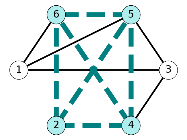
Definition 9.14 Given an undirected graph \(G = (V,E)\), we say that a subset \(S \subseteq V\) is a stable set if it consists of completely disconnected vertices: \[ \text{For all } \{i,j\} \in S, \;\; \{i,j\} \notin E. \]

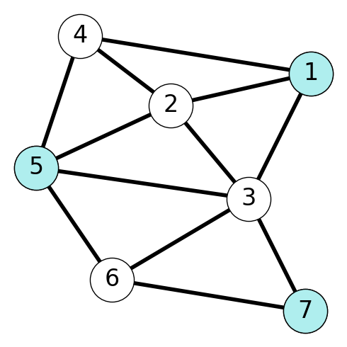
Example 9.7 Figure 9.3 illustrates the stable set \(\{1,5,7\}\) in the given graph: there are no edges between the nodes in the stable set. On the other hand, the set \(\{2,4,6\}\) is not stable because the given graph contains the edge \(\{2,4\}\).

9.5.4 The Stable Set Problem

Definition 9.15

STAB-d: Given an undirected graph \(G = (V,E)\) and integer \(L\), does \(G\) contain a stable set of size at least \(L\)?

Its optimization counterpart is

STAB: Given an undirected graph \(G=(V,E)\), find a stable set in \(G\) of maximum size.

9.5.5 3-SAT to STAB-d

We have used a reduction to show that 3-SAT is \(\mathbf{NP}\)-complete. Next, we want to reduce 3-SAT to STAB-d to show that STAB-d is \(\mathbf{NP}\)-complete. We have the following theorem.

Theorem 9.9 STAB-d is \(\mathbf{NP}\)-complete.

9.5.5.1 Membership in \(\mathbf{NP}\)

Any stable set with \(|S|\ge L\) is a polytime-verifiable certificate.

Indeed, we can check that

\(\{i,j\} \notin E\) for each \(i,j \in S\), and
\(|S| \ge L\)

in linear time in \((|V|, |E|)\).

9.5.5.2 3-SAT \(\le_T^P\) STAB-d

Given a 3-SAT instance, we build a STAB-d instance with

3 vertices per clause, one per literal, all adjacent.
- The vertices of each clause form a triangle.
An edge per pair of vertices whose literals represent the same variable but one is positive and the other is negative.
\(L = m\) the number of 3-SAT clauses.

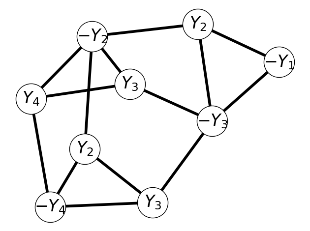
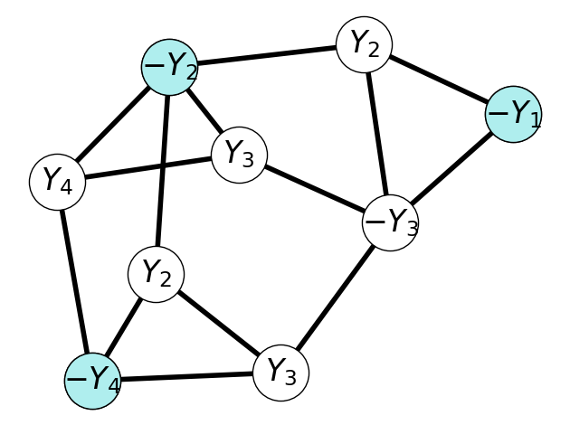
Example 9.8 Consider the following 3-SAT instance. \[ (−Y_1 \vee Y_2 \vee −Y_3) \wedge (Y_4 \vee −Y_2 \vee Y_3) \wedge (−Y_4 \vee Y_2 \vee Y_3). \] The corresponding instance of 3-SAT is given by the graph in Figure 9.4 with \(L = 3\). Here, we have three triangles/cycles corresponding to each of the three clauses.

Figure 9.4: STAB-d instance from 3-SAT instance

9.5.5.3 Establishing the Reduction

We want to show that 3-SAT is feasible if and only if STAB-d has answer YES. That is, there is a TA satisfying all clauses in the 3-SAT instance if and only if there is a stable set \(S\) in \(G\) with size at least \(L\).

We first establish necessity. To do so, note that, given a TA satisfying all clauses, we can construct a stable set \(S\) by choosing a single vertex from each triangle corresponding to either:

positive literal \(Y_i\) with \(Y_i = T\), or
negative literal \(-Y_i\) with \(Y_i = F\).

To illustrate this process, consider the 3-SAT instance from before: \[ (−Y_1 \vee Y_2 \vee −Y_3) \wedge (Y_4 \vee −Y_2 \vee Y_3) \wedge (−Y_4 \vee Y_2 \vee Y_3). \] This has TA: \((Y_1, Y_2, Y_3, Y_4) = (F, F, T, F)\).

Following the process above:

We add the node \(-Y_1\) from the triangle corresponding to \(C_1\) to \(S\);
We can pick \(-Y_2\) or \(Y_3\) from \(C_2\) to add; let’s pick \(-Y_2\);
Similarly, we can pick either \(Y_3\) or \(-Y_4\) from \(C_3\); let’s pick \(Y_3\).

This yields the stable set illustrated in Figure 9.5.

This process yields a stable set \(S\) with cardinality \(L=m\). Indeed, we have picked one node per triangle. Moreover, there are no inter-triangle edges, i.e., no edges between \(i,j \in S\) within triangles. Finally, note that we picked literals to construct \(S\) from a truth assignment. Thus, we cannot have \(Y_i\) and \(-Y_i\) both in \(S\), so there are no intra-triangle edges. Therefore, \(|S| = m = L\) and we have no edges between \(i,j\in S\). Therefore, \(S\) is a stable set with \(|S| \ge L\) and, hence this is a YES-instance of STAB-d.

We next prove sufficiency. Given stable set \(S\) of size \(L=m\), we can build a truth assignment.

For each triangle/clause \(C\), we set:

\(Y_i = T\) if the vertex in \(S \cap C\) is a vertex associated with positive literal \(Y_i\).
\(Y_i = F\) if the vertex in \(S \cap C\) is a vertex associated with a negative literal \(-Y_i\).

We set any remaining variable to either \(T\) or \(F\) (it makes no difference).

Returning to our earlier example, suppose that we have stable set given by Figure 9.6.

We can construct a truth assignment by setting \(Y_3 = F\), \(Y_2 = F\), and \(Y_4 = F\) (\(Y_1\) can be \(T\) or \(F\)).

In general, the truth assignment we build is consistent:

We cannot set \(Y_i = T\) and \(Y_i = F\) for some literal \(Y_i\).
If we could, then \(S\) would not be stable since we would have edge between \(Y_i\) and \(-Y_i\) in different clauses.

By construction, all clauses are satistfied and 3-SAT is a YES-instance if and only if the corresponding instance of STAB-d is a YES-instance.

9.5.6 Cliques

Definition 9.16 Given an undirected graph \(G=(V,E)\), a clique is a subset \(C\subseteq V\) of completely connected vertices: \[ \{i,j\} \in E \;\;\; \text{for all } i\neq j \in C. \]

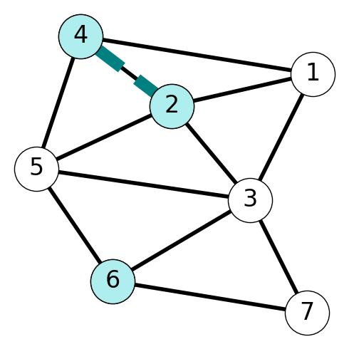
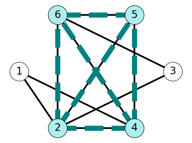
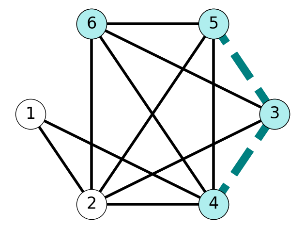
Example 9.9 Consider the graph \(G\) given in Figure 9.7. The set \(\{2,4,5,6\}\) is a clique since every node in this set is adjacent to every other node. On the other hand, the set \(\{3,4,5,6\}\) is not a clique since several pairs of nodes in this set are not adjacent, e.g., \(\{3,4\},\{3,5\} \notin E\).

9.5.7 The Maximum Clique Problem

Definition 9.17

CLIQUE: Given undirected graph \(G\), find a clique in \(G\) with maximum size.
CLIQUE-d: Given an undirected graph \(G=(V,E)\) and integer \(L\), does \(G\) have a clique of size \(\ge L\)?

Theorem 9.10 CLIQUE-d is \(\mathbf{NP}\)-complete.

9.5.7.1 Membership in \(\mathbf{NP}\)

Any clique \(C\) with \(|C| \ge L\) is a polytime-verifiable certificate.

Indeed, we require polynomially-many operations to check that

\(|C| \ge L\), and
\(\{i,j\} \in E\) for all \(i,j \in C\).

9.5.7.2 STAB-d \(\le_T^p\) CLIQUE-d

Let’s consider the complement graph \(\overline{G}\) of \(G\) where \[ \overline{G} = (V, \overline{E}) \text{ with } \overline{E}:= V\times V \setminus {E} \] (ignoring self-loops \(\{i,i\}\)). Alternately, if \(i\neq j\) then \(\{i,j\} \in \overline{E}\) if and only if \(\{i,j\} \notin E\).

Lemma 9.1 Cliques in \(\overline{G}\) are stable sets in \(G\) since \(\overline{E}\) is the complement of \({E}\).

The following theorem establishes equivalency of CLIQUE-d and STAB-d.

Theorem 9.11 \(\overline{G}\) contains a clique of size \(L\) if and only if \(G\) contains a stable set of size \(L\).

Theorem 9.11 establishes that STAB-d \(\le_T^P\) CLIQUE-d. Indeed, we have to the following algorithm for solving \(G\):

Given \(G\), \(L\).
Form \(\overline G\).
Use algorithm for CLIQUE-d to answer YES/NO for ``does \(\overline{G}\) have clique of size at least \(L\)?’’
Use this answer to return YES/NO to the original instance of STAB-d.